Using Statistics to Predict

http://evolve.elsevier.com/Grove/practice/

In nursing practice, the ability to predict future events is crucial. Clinical researchers might investigate if length of hospital stay of patients can be predicted by severity of illness. Health outcome researchers want to know what factors play an important role in responses of patients to health promotion, illness prevention, and rehabilitation interventions. Educators are interested in knowing what variables are most effective in predicting scores of undergraduate nurses on the registered nurse (RN) licensure examination. Advanced practice nurses are interested in what variables predict their success in passing their national certification examinations.

The statistical procedure most commonly used for prediction is regression analysis. The purpose of a regression analysis is to identify which factor or factors predict or explain the value of a dependent (outcome) variable. In some cases, the analysis is exploratory, and the focus is prediction. In others, selection of variables is based on a theoretical proposition, and the purpose is to develop an explanation that confirms the theoretical proposition.

In regression analysis, the independent (predictor) variable or variables influence variation or change in the value of the dependent variable. The goal is to determine how accurately one can predict the value of an outcome (or dependent) variable based on the value or values of one or more predictor (or independent) variables. This chapter describes some common statistical procedures used for prediction. These procedures include simple linear regression, multiple regression, logistic regression, and Cox proportional hazards regression.

Simple Linear Regression

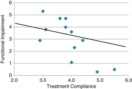
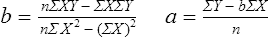
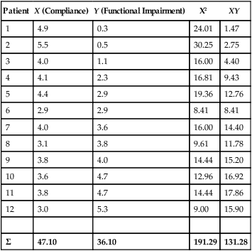
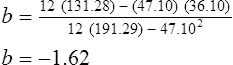
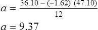
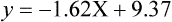
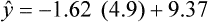
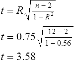
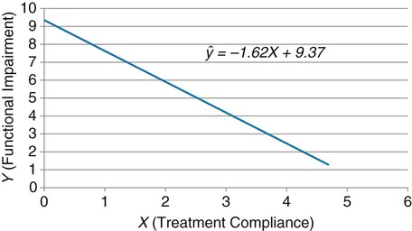
Simple linear regression provides a means to estimate the value of a dependent variable based on the value of an independent variable. Simple linear regression is an effort to explain the dynamics within the scatter plot by drawing a straight line (the line of best fit) through the plotted scores. This line is drawn to explain best the linear relationship or association between two variables. Knowing that linear relationship, we can, with some degree of accuracy, use regression analysis to predict the value of one variable if we know the value of the other variable (Cohen & Cohen, 1983). Figure 24-1 illustrates the linear relationship between treatment compliance (independent variable) and posttreatment functional impairment (dependent variable) among patients with chronic pain. As shown in the scatter plot, there is a strong inverse relationship between the two variables. Higher levels of treatment compliance are associated with lower levels of functional impairment.

Figure 24-1 Linear relationship between treatment compliance and posttreatment functional impairment.

In simple linear regression, the dependent variable is continuous, and the predictor can be any scale of measurement. However, if the predictor is nominal, it must be correctly coded. When the data are ready, the parameters a and b are computed to obtain a regression equation. To understand the mathematical process, recall the algebraic equation for a straight line:

y=bx+a

where

y = dependent variable (outcome)

x = independent variable (predictor)

b = slope of the line (beta, or what the increase in value is along the x-axis for every unit of increase in the y value)

a = y-intercept (the point where the regression line intersects the y-axis)

A regression equation can be generated with a data set containing participants’ x and y values. When this equation is generated, it can be used to predict y values of future participants, given only their x values. In simple or bivariate regression, predictions are made in cases with two variables. The score on variable y (dependent variable) is predicted from the same individual’s known score on variable x (independent variable).

No single regression line can be used to predict with complete accuracy every y value from every x value. You could draw an infinite number of lines through the scattered paired values. However, the purpose of the regression equation is to develop the line that allows the highest degree of prediction possible—the line of best fit. The procedure for developing the line of best fit is the method of least squares. The formulas for the beta (b) and y-intercept (a) of the regression equation are computed as follows. Note that when the b is calculated, that value is inserted into the formula for a.

b=nΣXY−ΣXΣYnΣX2−(ΣX)2a=ΣY−bΣXn

Calculation of Simple Linear Regression

Table 24-1 displays how one would arrange data to perform linear regression by hand. Regression analysis is conducted by a computer for most studies, but this calculation is provided to increase your understanding of the aspects of regression analysis and how to interpret the results. This example uses actual clinical data obtained from adults with a painful injury who received multidisciplinary pain management. The calculation in this chapter includes a subset of the study data belonging to those patients (n = 12) with the highest levels of coping skills (Cipher, Fernandez, & Clifford, 2002). A subset was selected for this illustration so that the computation example would be small and manageable. In actuality, studies involving linear regression need to be adequately powered, so they employ a larger sample (Aberson, 2010; Cohen & Cohen, 1983). The strength of this example is that the data are actual, unmodified clinical data from a study.

TABLE 24-1

Computation of Linear Regression Equation

Patient	X (Compliance)	Y (Functional Impairment)	X²	XY
1	4.9	0.3	24.01	1.47
2	5.5	0.5	30.25	2.75
3	4.0	1.1	16.00	4.40
4	4.1	2.3	16.81	9.43
5	4.4	2.9	19.36	12.76
6	2.9	2.9	8.41	8.41
7	4.0	3.6	16.00	14.40
8	3.1	3.8	9.61	11.78
9	3.8	4.0	14.44	15.20
10	3.6	4.7	12.96	16.92
11	3.8	4.7	14.44	17.86
12	3.0	5.3	9.00	15.90

Σ	47.10	36.10	191.29	131.28

The first variable in Table 24-1 is the patient’s level of treatment compliance—the predictor or independent variable (x) in this analysis. The second variable is the patient’s posttreatment level of functional impairment—the dependent variable (y). Treatment compliance was assessed by patients’ scores on the Cognitive Psychophysiological Treatment Clinical Rating Scales (Clifford, Cipher, & Schumacker, 2003), which yields an overall compliance score with higher numbers representing better levels of compliance with the pain management treatment regimen. Functional impairment was represented by patients’ scores on the Interference subscale of the Multidimensional Pain Inventory (Kerns, Turk, & Rudy, 1985), with higher scores representing more functional impairment. The null hypothesis being tested is: Treatment compliance is not a significant predictor of posttreatment functional impairment among patients undergoing pain management. The data in Table 24-1 are arranged in columns, which correspond to the elements of the formula. The summed values in the last row of Table 24-1 are inserted into the appropriate places in the formula.

Calculation Steps

Step 1: Calculate b.

From the values in Table 24-1, we know that n = 12, ΣX = 47.10, ΣY = 36.10, ΣX² = 191.29, and ΣXY = 131.28. These values are inserted into the formula for b, as follows:

b=12(131.28)−(47.10)(36.10)12(191.29)−47.102b=−1.62

Step 2: Calculate a.

From Step 1, we know that b = −1.62, and we plug this value into the formula for a:

a=36.10−(−1.62)(47.10)12a=9.37

Step 3: Write the new regression equation:

y=−1.62X+9.37

Step 4: Calculate R

The multiple R is defined as the correlation between the actual y values and the predicted y values using the new regression equation. The predicted y value using the new equation is represented by the symbol ŷ to differentiate it from y, which represents the actual y values in the data set. We can use our new regression equation from Step 3 to compute predicted functional impairment levels for each participant, the outcome of interest, using his or her compliance rating. For example, the compliance rating of patient no. 1 is 4.9, and the predicted functional impairment for patient no. 1 is calculated as:

yˆ=−1.62(4.9)+9.37

yˆ=1.43

The predicted ŷ is 1.43. This procedure would be continued for the rest of the subjects, and the Pearson correlation between the actual functional impairment levels (y) and the predicted functional impairment levels (ŷ) would yield the multiple R value. In this example, R = 0.75. The higher R, the more likely that the new regression equation accurately predicts y because the higher the correlation, the closer the actual y values are to the predicted ŷ values. Figure 24-2 displays the regression line where the x-axis represents possible treatment compliance values, and the y-axis represents the predicted functional impairment levels (ŷ values).

Figure 24-2 Regression line represented by regression equation.

Step 5: Determine whether the predictor variable significantly predicts y.

To know whether the predictor significantly predicts y, the value of beta must be tested against zero because zero reflects the presence of no significant association between the variables, or null hypothesis. In simple regression, this is most easily accomplished by using the R value from Step 4:

t=Rn−21−R2t=0.7512−21−0.56t=3.58

The t value is compared with the t probability distribution table (see Appendix B). The df for this t statistic is n − 2. The critical t value at alpha (α) = 0.05, df = 10 is 2.23. Our obtained t was 3.58, which exceeds the critical value in the table, indicating a significant association between the predictor (x) and outcome (y).

Step 6: Calculate R².

After establishing the statistical significance of the R value, it must be examined for clinical importance. This examination is accomplished by obtaining the coefficient of determination for regression—which simply involves squaring the R value. R² represents the percentage of variance in y explained by the predictor. In our example, R was 0.75, and R² was 0.56. Multiplying 0.56 × 100% indicates that 56% of the variance in posttreatment functional impairment can be explained by knowing the patients’ level of treatment compliance (Cohen & Cohen, 1983).

R² is most helpful in testing the contribution of the predictors in explaining an outcome when more than one predictor is included in the regression model. In contrast to R, R² for one regression model can be compared with another regression model that contains additional predictors (Cohen & Cohen, 1983). For example, Cipher et al. (2002) added another predictor, the patients’ coping style, to the regression model of functional impairment. The R² values of both models were compared, the first with treatment compliance as the sole predictor and the second with treatment compliance and copying style as predictors. The R² values of the two models were statistically compared to indicate whether the proportion of variance in ŷ was significantly increased by including the second predictor of coping style in the model.