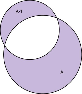
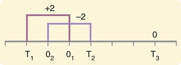
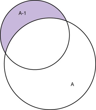
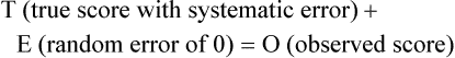
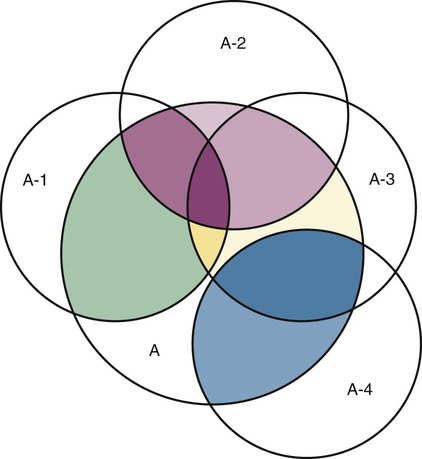
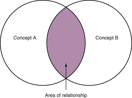
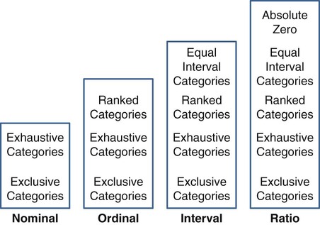
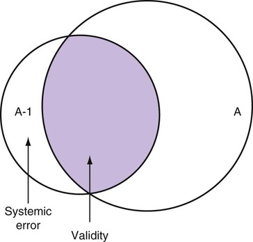
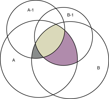
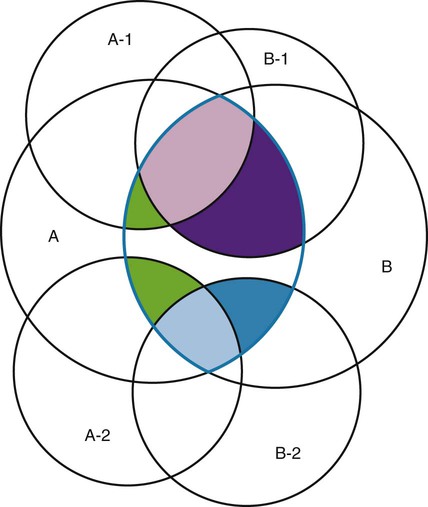
Measurement is the process of assigning numbers to objects, events, or situations in accord with some rule (Kaplan, 1963). The numbers assigned can indicate numerical values or categories for the objects being measured for research or practice. Instrumentation, a component of measurement, is the application of specific rules to develop a measurement device such as a scale or questionnaire. Quality instruments are essential for obtaining trustworthy data when measuring outcomes for research and practice (Doran, 2011; Melnyk & Fineout-Overhold, 2011; Waltz, Strickland, & Lenz, 2010). When measuring a subjective concept such as pain experienced by a child, researchers and nurses in practice need to use an instrument that captures the pain the child is experiencing. A commonly used scale to measure a child’s pain is the Wong-Baker FACES Pain Rating Scale (Hockenberry & Wilson, 2009). By using this valid and reliable rating scale to measure the child’s pain, any change in the measured value can be attributed to a change in the child’s pain rather than measurement error. A copy of the Wong-Baker FACES Pain Rating Scale is provided in Chapter 17. Selecting accurate and precise physiological measurement methods and valid and reliable scales and questionnaires is essential in measuring study variables and outcomes in practice (Bannigan & Watson, 2009; Bialocerkowski, Klupp, & Bragge, 2010; DeVon, et al., 2007). However, in nursing, the characteristic we want to measure often is an abstract idea or concept, such as pain, stress, depression, anxiety, caring, or coping. If the element to be measured is abstract, it is best clarified through a conceptual definition (see Chapter 8). The conceptual definition can be used to select or develop appropriate means of measuring the concept. The instrument or measurement strategy used in the study must match the conceptual definition. An abstract concept is not measured directly; instead, indicators or attributes of the concept are used to represent the abstraction. This is referred to as indirect measurement. For example, the complex concept of coping might be defined by the frequency or accuracy of identifying problems, the creativity in selecting solutions, and the speed or effectiveness in resolving the problem. A single measurement strategy rarely, if ever, can completely measure all aspects of an abstract concept. Multi-item scales have been developed to measure abstract concepts, such as the Spielberger State-Trait Anxiety Inventory developed to measure individuals’ innate anxiety trait and their anxiety in a specific situation (Spielberger, Gorsuch, & Lushene, 1970). There is also error in indirect measures. Efforts to measure concepts usually result in measuring only part of the concept or measures that identify an aspect of the concept but also contain other elements that are not part of the concept. Figure 16-1 shows a Venn diagram of the concept A measured by instrument A-1. In this figure, A-1 does not measure all of concept A. In addition, some of what A-1 measures is outside the concept of A. Both of these situations are examples of errors in measurement and are shaded in Figure 16-1. This equation is a means of conceptualizing random error and not a basis for calculating it. Because the true score is never known, the random error is never known but only estimated. Theoretically, the smaller the error score, the more closely the observed score reflects the true score. Therefore, using instruments that reduce error improves the accuracy of measurement (Waltz et al., 2010). Several factors can occur during the measurement process that can increase random error. These factors include (1) transient personal factors, such as fatigue, hunger, attention span, health, mood, mental status, and motivation; (2) situational factors, such as a hot stuffy room, distractions, the presence of significant others, rapport with the researcher, and the playfulness or seriousness of the situation; (3) variations in the administration of the measurement procedure, such as interviews in which wording or sequence of questions is varied, questions are added or deleted, or researchers code responses differently; and (4) processing of data, such as errors in coding, accidentally marking the wrong column, punching the wrong key when entering data into the computer, or incorrectly totaling instrument scores (Devon et al., 2007; Waltz et al., 2010). If you were to measure a variable for three subjects and diagram the random error, it might appear as shown in Figure 16-2. The difference between the true score of subject 1 (T1) and the observed score (O1) is two positive measurement intervals. The difference between the true score (T2) and observed score (O2) for subject 2 is two negative measurement intervals. The difference between the true score (T3) and observed score (O3) for subject 3 is zero. The random error for these three subjects is zero (+2 − 2 + 0 = 0). In viewing this example, one must remember that this is only a means of conceptualizing random error. Measurement error that is not random is referred to as systematic error. A scale that weighs subjects 3 pounds more than their true weights is an example of systematic error. All of the body weights would be higher, and, as a result, the mean would be higher than it should be. Systematic error occurs because something else is being measured in addition to the concept. A conceptualization of systematic error is presented in Figure 16-3. Systematic error (represented by the shaded area in the figure) is due to the part of A-1 that is outside of A. This part of A-1 measures factors other than A and biases scores in a particular direction. Another effective means of diminishing systematic error is to use more than one measure of an attribute or a concept and to compare the measures. To make this comparison, researchers use various data collection methods, such as scale, interview, and observation. Campbell and Fiske (1959) developed a technique of using more than one method to measure a concept, referred to as the multimethod-multitrait technique. More recently, the technique has been described as a version of mixed methodology, as discussed in Chapter 10. These techniques allow researchers to measure more dimensions of abstract concepts, and the effect of the systematic error on the composite observed score decreases. Figure 16-4 illustrates how more dimensions of concept A are measured through the use of four instruments, designated A-1, A-2, A-3, and A-4. For example, a researcher could decrease systematic error in measures of anxiety by (1) administering the Spielberger State-Trait Anxiety Inventory, (2) recording blood pressure readings, (3) asking the subject about anxious feelings, and (4) observing the subject’s behavior. Multimethod measurement strategies decrease systematic error by combining the values in some way to give a single observed score of anxiety for each subject. However, sometimes it may be difficult logically to justify combining scores from various measures, and a mixed-methods approach might be the most appropriate to use in the study. Mixed-methods study uses a combination of quantitative and qualitative approaches in their implementation (Creswell, 2009). In some studies, researchers use instruments to examine relationships. Consider a hypothesis that tests the relationship between concept A and concept B. In Figure 16-5, the shaded area enclosed in the dark lines represents the true relationship between concepts A and B, such as the relationship between anxiety and depression. For example, two instruments, A-1 (Spielberger State Anxiety Scale) and B-1 (Center for Epidemiological Studies Depression Scale, Radloff, 1977), are used to examine the relationship between concepts A and B. The part of the true relationship actually reflected by A-1 and B-1 measurement methods is represented by the colored area in Figure 16-6. Because two instruments provide a more accurate measure of concepts A and B, more of the true relationship between concepts A and B can be measured. If additional instruments (A-2 and B-2) are used to measure concepts A and B, more of the true relationship might be reflected. Figure 16-7 demonstrates with different colors the parts of the true relationship between concepts A and B that is measured when concept A is measured with two instruments (A-1 and A-2) and concept B is measured with two instruments (B-1 and B-2). Figure 16-8 provides a summary for the rules for the four levels of measurement—nominal, ordinal, interval, and ratio. Data such as ethnicity, gender, marital status, religion, and diagnoses are examples of nominal data. When data are coded for entry into the computer, the categories are assigned numbers. For example, gender may be classified as 1 = male and 2 = female. The numbers assigned to categories in nominal measurement are used only as labels and cannot be used for mathematical calculations. Data that can be measured at the ordinal level can be assigned to categories of an attribute that can be ranked. There are rules for how one ranks data. As with nominal-scale data, the categories must be exclusive and exhaustive. With ordinal level data, the quantity of the attribute possessed can be identified. However, it cannot be shown that the intervals between the ranked categories are equal (see Figure 16-8). Ordinal data are considered to have unequal intervals. Scales with unequal intervals are sometimes referred to as ordered metric scales. In interval level of measurement, distances between intervals of the scale are numerically equal. Such measurements also follow the previously mentioned rules: mutually exclusive categories, exhaustive categories, and rank ordering. Interval scales are assumed to be a continuum of values (see Figure 16-8). The researcher can identify the magnitude of the attribute much more precisely. However, it is impossible to provide the absolute amount of the attribute because of the absence of a zero point on the interval scale. Ratio level of measurement is the highest form of measure and meets all the rules of the lower forms of measures: mutually exclusive categories, exhaustive categories, rank ordering, equal spacing between intervals, and a continuum of values. In addition, ratio level measures have absolute zero points (see Figure 16-8). Weight, length, and volume are common examples of ratio scales. Each has an absolute zero point, at which a value of zero indicates the absence of the property being measured: Zero weight means the absence of weight. In addition, because of the absolute zero point, one can justifiably say that object A weighs twice as much as object B, or that container A holds three times as much as container B. Laboratory values are also an example of ratio level of measurement where the individual with a fasting blood sugar (FBS) of 180 has an FBS twice that of an individual with a normal FBS of 90. To help expand understanding of levels of measurement (nominal, ordinal, interval, and ratio) and to apply this knowledge, Grove (2007) developed a statistical workbook focused on examining the levels of measurement, sampling methods, and statistical results in published studies. An important rule of measurement is that one should use the highest level of measurement possible. For example, you can collect data on age (measured) in a variety of ways: (1) you can obtain the actual age of each subject (ratio level of measurement); (2) you can ask subjects to indicate their age by selecting from a group of categories, such as 20 to 29, 30 to 39, and so on (ordinal level of measurement); or (3) you can sort subjects into two categories of younger than 65 years of age and 65 years of age and older (nominal level of measurement). The highest level of measurement in this case is the actual age of each subject, which is the preferred way to collect these data. If you need age categories for specific analyses in your research, the computer can be instructed to create age categories from the initial age data (Waltz et al., 2010). The level of measurement is associated with the types of statistical analyses that can be performed on the data. Mathematical operations are limited in the lower levels of measurement. With nominal levels of measurement, only summary statistics, such as frequencies, percentages, and contingency correlation procedures, can be used. However, if a variable such as age is measured at the ratio level (actual age of the subject), the data can be analyzed with more sophisticated analysis techniques. Variables measured at the interval or ratio level can be analyzed with the strongest statistical techniques available, which are more effective in identifying relationships among variables or determining differences between groups (Corty, 2007; Grove, 2007). There is controversy over the system that is used to categorize measurement levels, dividing researchers into two factions: fundamentalists and pragmatists. Pragmatists regard measurement as occurring on a continuum rather than by discrete categories, whereas fundamentalists adhere rigidly to the original system of categorization (Nunnally & Bernstein, 1994; Stevens, 1946). The primary focus of the controversy relates to the practice of classifying data into the categories ordinal and interval. This controversy developed because, according to the fundamentalists, many of the current statistical analysis techniques can be used only with interval and ratio data. Many pragmatists believe that if researchers rigidly adhered to rules developed by Stevens (1946), few if any measures in the social sciences would meet the criteria to be considered interval-level data. They also believe that violating Stevens’ criteria does not lead to serious consequences for the outcomes of data analysis. Pragmatists often treat ordinal data from multi-item scales as interval data, using statistical methods (parametric analysis techniques) to analyze them, such as Pearson’s product-moment correlation coefficient, t-test, and analysis of variance (ANOVA), which are traditionally reserved for interval or ratio level data (Armstrong, 1981; Knapp, 1990). Fundamentalists insist that the analysis of ordinal data be limited to statistical procedures designed for ordinal data, such as nonparametric procedures. Parametric statistical analysis techniques were developed to analyze interval and ratio level data, and nonparametric techniques were developed to analyze nominal and ordinal data (see Chapter 21). The Likert scale uses scale points such as “strongly disagree,” “disagree,” “uncertain,” “agree,” and “strongly agree.” Numerical values (e.g., 1, 2, 3, 4, and 5) are assigned to these categories. Fundamentalists claim that equal intervals do not exist between these categories. It is impossible to prove that there is the same magnitude of feeling between “uncertain” and “agree” as there is between “agree” and “strongly agree.” Therefore, they hold this is ordinal level data, and parametric analyses cannot be used. Pragmatists believe that with many measures taken at the ordinal level, such as scaling procedures, an underlying interval continuum is present that justifies the use of parametric statistics (Knapp, 1990; Nunnally & Bernstein, 1994). Our position agrees more with the pragmatists than with the fundamentalists. Many nurse researchers analyze data from Likert scales and other rating scales as though the data were interval level (Waltz et al., 2010). However, some of the data in nursing research are obtained through the use of crude measurement methods that can be classified only into the lower levels of measurement (ordinal or nominal). Therefore, we have included the nonparametric statistical procedures needed for their analysis in Chapters 22 to 25 on statistics. Referencing involves comparing a subject’s score against a standard. Two types of testing involve referencing: norm-referenced testing and criterion-referenced testing. Norm-referenced testing addresses the question, “How does the average person score on this test or instrument?” This testing involves standardization of scores for an instrument that is accomplished by data collection over several years, with extensive reliability and validity information available on the instrument. Standardization involves collecting data from thousands of subjects expected to have a broad range of scores on the instrument. From these scores, population parameters such as the mean and standard deviation (described in Chapter 22) can be developed. Evidence of the reliability and validity of the instrument can also be evaluated through the use of the methods described later in this chapter. The best-known norm-referenced test is the Minnesota Multiphasic Personality Inventory (MMPI), which is used commonly in psychology and occasionally in nursing research and practice to diagnosis personality disorders. The Graduate Record Examination (GRE) is another norm-referenced test commonly used as one of the admission criteria for graduate study. Criterion-referenced testing asks the question, “What is desirable in the perfect subject?” It involves comparing a subject’s score with a criterion of achievement that includes the definition of target behaviors. When the subject has mastered these behaviors, he or she is considered proficient in the behavior (DeVon et al., 2007; Sax, 1997). The criterion might be a level of knowledge or desirable patient outcomes. Criterion measures have been used for years to evaluate outcomes in healthcare agencies and to determine clinical expertise of students. For example, a clinical evaluation form would include the critical behaviors the nurse practitioner (NP) student is expected to master in a pediatric course to be clinically competent to care for pediatric patients at the end of the course. Criterion-reference testing is also used in nursing research. Criterion-referenced testing might be used to measure the clinical expertise of a nurse or the self-care of a cardiac patient after cardiac rehabilitation. The reliability of an instrument denotes the consistency of the measures obtained of an attribute, item, or situation in a study or clinical practice. The greater the reliability or consistency of the measures of a particular instrument, the less random error in the measurement method (Bannigan & Watson, 2009; Bialocerkowski et al., 2010; DeVon et al., 2007). If the same measurement scale is administered to the same individuals at two different occasions, the measurement is reliable if the individuals’ responses to the items remain the same (assuming that nothing has occurred to change their responses). For example, if you use a scale to measure the anxiety levels of 10 individuals at two points in time 30 minutes apart, you would expect the individuals’ anxiety levels to be relatively unchanged from one measurement to the next if the scale is reliable. If two data collectors observe the same event and record their observations on a carefully designed data collection instrument, the measurement would be reliable if the recordings from the two data collectors are comparable. The equivalence of their results would indicate the reliability of the measurement technique. If responses vary each time a measure is performed, there is a chance that the instrument is unreliable, meaning that it yields data with a large random error. Reliability plays an important role in the selection of measurement methods for use in a study. Researchers need instruments that are reliable and provide values with only a small amount of error. Reliable instruments enhance the power of a study to detect significant differences or relationships actually occurring in the population under study. It is important to examine the reliability of an instrument from previous research before using it in a study. Estimates of instrument reliability are specific to the population and sample being studied. High reported reliability values on an established instrument do not guarantee that its reliability would be satisfactory in another sample from a different population (Waltz et al., 2010). Researchers need to perform reliability testing on each instrument used in their study before performing other statistical analyses. The reliability values must be included in the published report of a study to document that the instruments used were reliable for the study sample (Bialocerkowski et al., 2010; DeVon et al., 2007). Reliability testing examines the amount of measurement error in the instrument being used in a study. Reliability is concerned with the dependability, consistency, stability, precision, reproducibility, and comparability of a measurement method (Bartlett & Frost, 2008). The strongest measure of reliability is obtained from heterogeneous samples versus homogeneous samples. Heterogeneous samples have more between-participant variability, and this is a stronger evaluation of reliability than homogeneous samples with little between-participant variation. When critically appraising the reliability of an instrument in a study, you need to examine the sample for heterogeneity by determining the variability of the scores among study participants (Bartlett & Frost, 2008; Bialocerkowski et al., 2010). All measurement techniques contain some random error, and the errors might be due to the measurement method used, the study participants, or the researchers gathering the data. Reliability exists in degrees and is usually expressed as a form of correlation coefficient, with 1.00 indicating perfect reliability and 0.00 indicating no reliability (Bialocerkowski et al., 2010). For example, reliability coefficients of 0.80 or higher are considered strong values for an established psychosocial scale such as the State-Trait Anxiety Inventory by Spielberger et al. (1970). With test-retest, the closer that reliability coefficient is to 1.00, the more stable the measurement method. The reliability coefficient varies based on the type of reliability being examined. The three most common types of reliability discussed in healthcare studies are (1) stability reliability, (2) equivalence reliability, and (3) internal consistency (Bannigan & Watson, 2009; Bialocerkowski et al., 2010; DeVon et al., 2007; Waltz et al., 2010). The optimal time period between test-retest measurements depends on the variability of the variable being measured, complexity of the measurement process, and characteristics of the participants (Bialocerkowski et al., 2010). Physical measures and equipment can be tested and then immediately retested, or the equipment can be used for a time and then retested to determine the necessary frequency of recalibration. For example, in measuring blood pressure (BP), researchers often take two to three BP readings 5 minutes apart and average the readings to obtain a reliable or precise measure of BP. Researchers can follow the standards for recalibration of equipment or be more conservative. The standard requirements might be to recalibrate the BP equipment every 6 months, but researchers might choose to recalibrate the equipment every month or even every week if multiple BP readings are being taken each day for a study. The test-retest of a measurement method might have a longer period of time if the variable being measured changes slowly. For example, the diagnosis of osteoporosis is made by bone mineral density (BMD) study of the hip, spine, and wrist. The BMD score is determined with a dual-energy x-ray absorptiometry (DEXA) scan. Because the BMD does not change rapidly in people even with treatment, test-retest over a 1- to 2-month time period could be used to show reliable or consistent DEXA scan scores for patients. With paper-and-pencil educational tests, a period of 2 to 4 weeks is recommended between the two testing times, but the time period for retesting does depend on what is measured and the instrument used (Sax, 1997). After the same participants have been retested with the same instrument, the investigators perform a correlational analysis on the scores from the two measurement times. This correlation is called the coefficient of stability, and the closer the coefficient is to 1.00, the more stable the instrument (Waltz et al., 2010). For some scales, test-retest reliability has not been as effective as originally anticipated. The procedure presents numerous problems. Subjects may remember their responses from the first testing time, leading to overestimation of the reliability. Subjects may be changed by the first testing and may respond to the second test differently, leading to underestimation of the reliability (Bialocerkowski et al., 2010). Test-retest reliability requires the assumption that the factor being measured has not changed between the measurement points. Many of the phenomena studied in nursing, such as hope, coping, pain, and anxiety, do change over short intervals. Thus, the assumption that if the instrument is reliable, values will not change between the two measurement periods may not be justifiable. If the factor being measured does change, the test is not a measure of reliability. If the measures stay the same even though the factor being measured has changed, the instrument may lack reliability. If researchers are going to examine the reliability of an instrument with test-retest, they need to determine the optimum time between administrations of the instrument based on the variable being measured and the study participants (Devon et al., 2007). Stability of a measurement method is important and needs to be examined as part of instrument development and discussed when the instrument is used in a study. When describing test-retest results, researchers need to discuss the process and the time period between administering an instrument and the rationale for this time frame. If a scale was administered twice 30 minutes apart or there was 1 month between test and retesting, the consistency of the subjects’ scores need to be discussed in terms of the timing for retesting (Bannigan & Watson, 2009; Bialocerkowski et al., 2010; DeVon et al., 2007). Equivalence reliability compares two versions of the same paper-and-pencil instrument or two observers measuring the same event. Comparison of two observers is referred to as interrater reliability. Comparison of two paper-and-pencil instruments is referred to as alternate-forms reliability or parallel-forms reliability. Alternative forms of instruments are of more concern in the development of normative knowledge testing. However, when repeated measures are part of the design, alternative forms of measurement, although not commonly used, would improve the design. Demonstrating that one is actually testing the same content in both tests is extremely complex, and the procedure is rarely used in clinical research (Bialocerkowski et al., 2010). The procedure for developing parallel forms involves using the same objectives and procedures to develop two like instruments. These two instruments when completed by the same group of study participants on the same occasion or two different occasions should have approximately equal means and standard deviations. In addition, these two instruments should correlate equally with another variable. For example, if two instruments were developed to measure pain, the scores from these two scales should correlate equally with perceived anxiety score. If both forms of the instrument are administered during the same occasion, a reliability coefficient can be calculated to determine equivalence. A coefficient of 0.80 or higher indicates equivalence (Waltz et al., 2010). Determining interrater reliability is a concern when studies include observational measurement, which is common in qualitative research. Interrater reliability values need to be reported in any study in which observational data are collected or judgments are made by two or more data gatherers. Two techniques determine interrater reliability. Both techniques require that two or more raters independently observe and record the same event using the protocol developed for the study or that the same rater observes and records an event on two occasions. To judge interrater reliability adequately, the raters need to observe at least 10 subjects or events (DeVon et al., 2007; Waltz et al., 2010). A digital recorder can be used to record the raters to determine their consistency in recording essential study information. Every data collector used in the study must be tested for interrater reliability and trained to a consistency in data collection. When raters know they are being watched, their accuracy and consistency are considerably better than when they believe they are not being watched. Interrater reliability declines (sometimes dramatically) when the raters are assessed covertly (Topf, 1988). You can develop strategies to monitor and reduce the decline in interrater reliability, but they may entail considerable time and expense. Tests of instrument internal consistency or homogeneity, used primarily with paper-and-pencil tests or scales, address the correlation of various items within the instrument. The original approach to determining internal consistency was split-half reliability. This strategy was a way of obtaining test-retest reliability without administering the test twice. The instrument items were split in odd-even or first-last halves, and a correlational procedure was performed between the two halves. In the past, researchers generally reported the Spearman-Brown correlation coefficient in their studies (Nunnally & Bernstein, 1994; Sax, 1997). One of the problems with the procedure was that although items were usually split into odd-even items, it was possible to split them in a variety of ways. Each approach to splitting the items would yield a different reliability coefficient. The researcher could continue to split the items in various ways until a satisfactorily high coefficient was obtained. More recently, testing the internal consistency of all the items in the instrument has been seen as a better approach to determining reliability. Although the mathematics of the procedure are complex, the logic is simple. One way to view it is as though one conducted split-half reliabilities in all the ways possible and then averaged the scores to obtain one reliability score. Internal consistency testing examines the extent to which all the items in the instrument consistently measure a concept. Cronbach’s alpha coefficient is the statistical procedure used for calculating internal consistency for interval and ratio level data. This reliability coefficient is essentially the mean of the interitem correlations and can be calculated using most data analysis programs such as the Statistical Program for the Social Sciences (SPSS). If the data are dichotomous, such as a symptom list that has responses of present or absent, the Kuder-Richardson formulas (KR 20 or KR 21) can be used to calculate the internal consistency of the instrument (DeVon et al., 2007). The KR 21 assumes that all the items on a scale or test are equally difficult; the KR 20 is not based on this assumption. Waltz et al. (2010) provided the formulas for calculating both KR 20 and KR 21. Cronbach’s alpha coefficients can range from 0.00, indicating no internal consistency or reliability, to 1.00, indicating perfect internal reliability with no measurement error. Alpha coefficients of 1.00 are not obtained in study results because all instruments have some measurement error. However, many respected psychosocial scales used for 15 to 30 years to measure study variables in a variety of populations have strong 0.8 or greater internal reliability coefficients. The coefficient of 0.80 (or 80%) indicates the instrument is 80% reliable with 20% random error (DeVon et al., 2007; Fawcett & Garity, 2009; Grove, 2007). Scales with 20 or more items usually have stronger internal consistency coefficients than scales with 10 to 15 items or less. Often scales that measure complex constructs such as quality of life (QOL) have subscales that measure different aspects of QOL, such as health, physical functioning, and spirituality. Some of these complex scales with distinct subscales, such as the QOL scale, might have lower Cronbach’s alpha coefficients since the scale is measuring different aspects of QOL. The subscales have fewer items than the total scale and usually lower Cronbach’s alpha coefficients but do need to show internal consistency in measuring a concept (Bialocerkowski et al., 2010; Waltz et al., 2010). Newer instruments, developed in the last 5 years, might show moderate internal reliability (0.70 to 0.79) when used in measuring variables in a variety of samples. The subscales of these new instruments might have internal reliability from 0.60 to 0.69. The authors of these scales might continue to refine them based on additional reliability and validity information to improve the reliability of the total scale and subscales. Reliability coefficients less than 0.60 are considered low and indicate limited instrument reliability or consistency in measurement with high random error. Higher levels of reliability or precision (0.90 to 0.99) are important for physiological measures that are used to determine critical physiological functions such as arterial pressure and oxygen saturation (Bialocerkowski et al., 2010; DeVon et al., 2007). The quality of the instrument reliability needs to be examined in terms of the type of study, measurement method, and population (DeVon et al., 2007; Kerlinger & Lee, 2000). In published studies, researchers need to identify the reliability coefficients of an instrument from previous research and for their particular study. Because the reliability of an instrument can vary from one population or sample to another, it is important that the reliability of the scale and subscales be determined and reported for the sample in each study (Bialocerkowski, et al., 2010). Dickerson, Kennedy, Wu, Underhill, and Othman (2010) conducted a study of QOL and anxiety levels of patients with implantable defibrillators. They provided the following discussion of the reliability of the scales they used in their study. Dickerson et al. (2010) used two very reliable scales to measure their study variables and documented this in their article. They measured anxiety with the Spielberger STAI, which was developed more than 40 years ago (Spielberger et al., 1970), has shown strong internal consistency in previous research (median alpha = 0.93), and was reliable in this study (Cronbach’s alpha = 0.90 to 0.96). In previous studies, the QLI: CV had strong internal consistency for the total scale (alpha = 0.90-0.95) and stability reliability with test-retest over 2 weeks and 1 month. In addition to the strong stability reliability coefficients, the researchers also provided the time frames for the test-retests that were run on the scale. Another strength is that the QLI: CV showed strong internal consistency for the total scale (alpha = 0.95 to 0.96) and the four subscales (alpha = 0.88 to 0.94) with the population in this study. Other approaches to testing internal consistency are (1) Cohen’s kappa statistic, which determines the percentage of agreement with the probability of chance being taken out; (2) correlating each item with the total score for the instrument; and (3) correlating each item with each other item in the instrument. This procedure, often used in instrument development, allows researchers to identify items that are not highly correlated and delete them from the instrument. Factor analysis may also be used to develop instrument reliability. The number of factors being measured influences the reliability of the instrument, and total instrument scores may be more reliable than the scores of the subscales. After performing the factor analysis, the researcher can delete instrument items with low factor weights. After these items have been deleted, reliability scores on the instrument are higher. For instruments with more than one factor, correlations can be performed between items and factor scores (see Chapter 23 for a discussion of factor analysis). It is essential that an instrument be both reliable and valid for measuring a study variable in a population. If the instrument has low reliability values, it cannot be valid because its measurement is inconsistent and has high measurement error (DeVon et al., 2007; Waltz et al., 2010). An instrument that is reliable cannot be assumed to be valid for a particular study or population. You need to determine the validity of the instrument you are using for your study, which you can accomplish in a variety of ways. The validity of an instrument determines the extent to which it actually reflects or is able to measure the construct being examined. Several types of validity are discussed in the literature, such as content validity, predictive validity, criterion validity, and construct validity. Within each of these types, subtypes have been identified. These multiple types of validity are very confusing, especially because the types are not discrete but are interrelated (Bannigan & Watson, 2009; DeVon et al., 2007; Fawcett & Garity, 2009). In this text, validity is considered a single broad measurement evaluation that is referred to as construct validity and includes various types, such as content validity, validity from factor analysis, convergent and divergent validity, validity from contrasting groups, and validity from prediction of future and current events (DeVon et al., 2007). All of the previously identified types of validity are now considered evidence of construct validity. In 1999, in its Standards for Educational and Psychological Testing, the American Psychological Association’s Committee to Develop Standards published standards used to judge the evidence of validity. This important work greatly extends our understanding of what validity is and how to achieve it. According to the American Psychological Association’s Committee to Develop Standards (1999), validity addresses the appropriateness, meaningfulness, and usefulness of the specific inferences made from instrument scores. It is the inferences made from the scores, not the scores themselves, that are important to validate (Devon et al., 2007; Goodwin & Goodwin, 1991). Validity, similar to reliability, is not an all-or-nothing phenomenon but rather a matter of degree. No instrument is completely valid. One determines the degree of validity of a measure rather than whether or not it has validity. Determining the validity of an instrument often requires years of work. Many authors equate the validity of the instrument with the rigorousness of the researcher. The assumption is that because the researcher develops the instrument, the researcher also establishes the validity. However, this is an erroneous assumption because validity is not a commodity that researchers can purchase with techniques. Validity is an ideal state—to be pursued, but not to be attained. As the roots of the word imply, validity includes truth, strength, and value. Some authors might believe that validity is a tangible “resource,” which can be acquired by applying enough appropriate techniques. However, we reject this view and believe measurement validity is similar to integrity, character, or quality, to be assessed relative to purposes and circumstances and built over time by researchers conducting a variety of studies (Brinberg & McGrath, 1985). Figure 16-9 illustrates validity (the shaded area) by the extent to which the instrument A-1 reflects concept A. As measurement of the concept improves, validity improves. The extent to which the instrument A-1 measures items other than the concept is referred to as systematic error (identified as the unshaded area of A-1 in Figure 16-9). As systematic error decreases, validity increases.
Measurement Concepts
 http://evolve.elsevier.com/Grove/practice/
Directness of Measurement
Measurement Error
Types of Measurement Errors


Levels of Measurement
Nominal Level of Measurement
Ordinal Level of Measurement
Interval Level of Measurement
Ratio Level of Measurement
Importance of Level of Measurement for Statistical Analyses
Controversy over Measurement Levels
Reference Testing of Measurement
Reliability
Stability Reliability
Equivalence Reliability

Internal Consistency
Validity
![]()
Stay updated, free articles. Join our Telegram channel

Full access? Get Clinical Tree


Nurse Key
Fastest Nurse Insight Engine
Get Clinical Tree app for offline access
