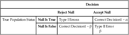
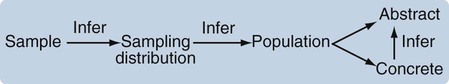
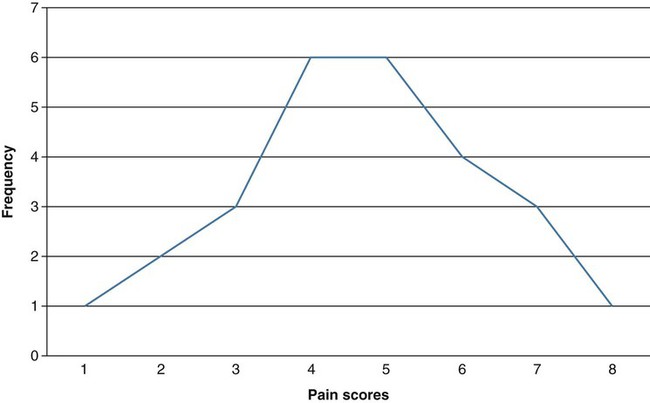
Data analysis is often considered one of the most exciting steps of the research process. During this phase, you will finally obtain answers to the questions that led to the development of your study. Nevertheless, nurses probably experience greater anxiety about this phase of the research process than any other, as they question issues that range from their knowledge about critically appraising published studies to their ability to conduct research. Critical appraisal of the results section of a quantitative study requires you to be able to (1) identify the statistical procedures used; (2) judge whether these statistical procedures were appropriate for the hypotheses, questions, or objectives of the study and for the data available for analysis; (3) comprehend the discussion of data analysis results; (4) judge whether the author’s interpretation of the results is appropriate; and (5) evaluate the clinical importance of the findings (see Chapter 18 for more details on critical appraisal). Critical appraisal of the results of studies and statistical analyses both require an understanding of the statistical theory underlying the process of analysis. This chapter and the following four chapters provide you with the information needed for critical appraisal of the results sections of published studies and for performance of statistical procedures to analyze data in studies and in clinical practice. This chapter introduces the concepts of statistical theory and discusses some of the more pragmatic aspects of quantitative data analysis: the purposes of statistical analysis, the process of performing data analysis, the method for choosing appropriate statistical analysis techniques for a study, and resources for conducting statistical analysis procedures. Chapter 22 explains the use of statistics for descriptive purposes, such as describing the study sample or variables. Chapter 23 focuses on the use of statistics to examine proposed relationships among study variables, such as the relationships among the variables dyspnea, anxiety, and quality of life. Chapter 24 explores the use of statistics for prediction, such as using independent variables of age, gender, cholesterol values, and history of hypertension to predict the dependent variable of cardiac risk level. Chapter 25 guides you in using statistics to determine differences between groups, such as determining the difference in muscle strength and falls (dependent variables) between an experimental or intervention group receiving a strength training program (independent variable) and a comparison group receiving standard care. One reason nurses tend to avoid statistics is that many were taught the mathematical mechanics of calculating statistical formulas and were given little or no explanation of the logic behind the analysis procedure or the meaning of the results (Grove, 2007). This mathematical process is usually performed by computer, and information about it offers little assistance to the individuals making statistical decisions or explaining results. We approach data analysis from the perspective of enhancing your understanding of the meaning underlying statistical analysis. You can use this understanding either for critical appraisal of studies or for conducting data analyses. Probability theory addresses statistical analysis as the likelihood of accurately predicting an event or the extent of an effect. Nurse researchers might be interested in the probability of a particular nursing outcome in a particular patient care situation. For example, what is the probability of patients older than 75 years of age with cardiac conditions falling when hospitalized? With probability theory, you could determine how much of the variation in your data could be explained by using a particular statistical analysis. In probability theory, the researcher interprets the meaning of statistical results in light of his or her knowledge of the field of study. A finding that would have little meaning in one field of study might be important in another (Good, 1983; Kerlinger & Lee, 2000). Probability is expressed as a lowercase p, with values expressed as percentages or as a decimal value ranging from 0 to 1. For example, if the exact probability is known to be 0.23, it would be expressed as p = 0.23. The p in statistics is defined as the probability of rejecting the null hypothesis when the null is actually true. Nurse researchers typically consider a p = 0.05 value or less to indicate a real effect. 1. State your primary null hypothesis. (Chapter 8 discusses the development of the null hypothesis.) 2. Set your study alpha (Type I error); this is usually α = 0.05. 3. Set your study beta (Type II error); this is usually β = 0.20. 4. Conduct power analyses (Aberson, 2010; Cohen, 1988). 5. Design and conduct your study. 6. Compute the appropriate statistic on your obtained data. 7. Compare your obtained statistic with its corresponding theoretical distribution in the tables provided in the Appendices at the back of this book. For example, if you analyzed your data with a t-test, you would compare the t value from your study with the critical values of t in the table. 8. If your obtained statistic exceeds the critical value in the distribution table, you can reject your null hypothesis. If not, you must accept your null hypothesis. These ideas are discussed in more depth in Chapters 23 through 25 when the results of statistics are presented. Cox (1958, p. 159) stated, “Significance tests, from this point of view, measure the adequacy of the data to support the qualitative conclusion that there is a true effect in the direction of the apparent difference.” Thus, the decision is a judgment and can be in error. The level of statistical significance attained indicates the degree of uncertainty in taking the position that the difference between the two groups is real. Classical hypothesis testing has been largely criticized for such errors in judgments (Cohen, 1994; Loftus 1993). Much emphasis has been placed on researchers providing indicators of effect, rather than just relying on p values, specifically, providing the magnitude of the obtained effect (e.g., a difference or relationship) as well as confidence intervals associated with the statistical findings. These additional statistics give consumers of research more information about the phenomenon being studied (Cohen 1994). We choose the probability of making a Type I error when we set alpha, and if we decrease the probability of making a Type I error, we increase the probability of making a Type II error. The relationships between Type I and Type II errors are defined in Table 21-1. Type II error occurs as a result of some degree of overlap between the values of different populations, so in some cases a value with a greater than 5% probability of being within one population may be within the dimensions of another population. TABLE 21-1 As stated in the steps of classical hypothesis testing previously, step 4 is “conducting a power analysis.” Power analysis involves determining the required sample size needed to conduct your study after performing steps 1, 2, and 3. Cohen (1988) identified four parameters of power: (1) significance level, (2) sample size, (3) effect size, and (4) power (standard of 0.80). If three of the four are known, the fourth can be calculated by using power analysis formulas. Significance level and sample size are straightforward. Chapter 15 provides a detailed discussion of determining sample size in quantitative studies that includes power analysis. Effect size is “the degree to which the phenomenon is present in the population or the degree to which the null hypothesis is false” (Cohen, 1988, pp. 9-10). For example, suppose you were measuring changes in anxiety levels, measured first when the patient is at home and then just before surgery. The effect size would be large if you expected a great change in anxiety. If you expected only a small change in the level of anxiety, the effect size would be small. Small effect sizes require larger samples to detect these small differences (see Chapter 15 for a detailed discussion of effect size). If the power is too low, it may not be worthwhile conducting the study unless a large sample can be obtained because statistical tests are unlikely to detect differences or relationships that exist. Deciding to conduct a study in these circumstances is costly in time and money, frequently does not add to the body of nursing knowledge, and can lead to false conclusions. Power analysis can be conducted via hand calculations, computer software, or online calculators and should be performed to determine the sample size necessary for a particular study (Aberson, 2010). Power analysis can be calculated by using the free power analysis software G*Power (Faul, Erdfelder, Lang, & Buchner, 2007) or statistical software such as NCSS, SAS, and SPSS (Table 21-2). In addition, many free sample size calculators are available online that are easy to use and understand. If you have questions, you could consult a statistician. TABLE 21-2 Software Applications for Statistical Analysis The findings of a study can be statistically significant but may not be clinically important. For example, one group of patients might have a body temperature 0.1° F higher than that of another group. Data analysis might indicate that the two groups are statistically significantly different. However, the findings have little or no clinical importance because of the small difference in temperatures between groups. It is often important to know the magnitude of the difference between groups in studies. However, a statistical test that indicates significant differences between groups (e.g., a t-test) provides no information on the magnitude of the difference. The extent of the level of significance (0.01 or 0.0001) tells you nothing about the magnitude of the difference between the groups or the relationship between two variables. The magnitude of group differences can best be determined through calculating effect sizes and confidence intervals (see Chapters 22 through 25). Use of the terms statistic and parameter can be confusing because of the various populations referred to in statistical theory. A statistic, such as a mean ( For example, perhaps you are interested in the cholesterol levels of women in the United States. Your population is women in the United States. You cannot measure the cholesterol level of every woman in the United States; therefore, you select a sample of women from this population. Because you wish your sample to be as representative of the population as possible, you obtain your sample by using random sampling techniques (see Chapter 15). To determine whether the cholesterol levels in your sample are similar to those in the population, you must compare the sample with the population. One strategy would be to compare the mean of your sample with the mean of the entire population. However, it is highly unlikely that you know the mean of the entire population; you must make an estimate of the mean of that population. You need to know how good your sample statistics are as estimators of the parameters of the population. First, you make some assumptions. You assume that the mean scores of cholesterol levels from multiple, randomly selected samples of this population would be normally distributed. This assumption implies another assumption: that the cholesterol levels of the population will be distributed according to the theoretical normal curve—that difference scores and standard deviations can be equated to those in the normal curve. The normal curve is discussed later in this chapter. A basic yet important way to begin describing a sample is to create a frequency distribution of the variable or variables being studied. A frequency distribution is a plot of one variable, whereby the x-axis consists of the possible values of that variable, and the y-axis is the tally of each value. For example, if you assessed a sample for a variable such as pain using a visual analogue scale, and your subjects reported particular values for pain, you could create a frequency distribution as illustrated in Figure 21-1.
Introduction to Statistical Analysis
 http://evolve.elsevier.com/Grove/practice/
Concepts of Statistical Theory
Probability Theory
Classical Hypothesis Testing
Type I and Type II Errors
Decision
Reject Null
Accept Null
True Population Status
Null Is True
Type I Errorα
Correct Decision1 − α
Null Is False
Correct Decision1 − β
Type II Error
β
Statistical Power
Software Application
Website
NCSS (Number Cruncher Statistical System)
www.ncss.com
SPSS (Statistical Packages for the Social Sciences)
www.spss.com
SAS (Statistical Analysis System)
www.sas.com
S+
spotfire.tibco.com
Stata
www.stat.com
JMP
www.jmp.com
Statistical Significance versus Clinical Importance
Samples and Populations
 ), is a numerical value obtained from a sample. A parameter is a true (but unknown) numerical characteristic of a population. For example, µ is the population mean or arithmetic average. The mean of the sampling distribution (mean of samples’ means) can also be shown to be equal to µ. A numerical value that is the mean (
 ) of the sample is a statistic; a numerical value that is the mean of the population (µ) is a parameter (Barnett, 1982).
Descriptive Statistics
![]()
Stay updated, free articles. Join our Telegram channel

Full access? Get Clinical Tree


Introduction to Statistical Analysis
Get Clinical Tree app for offline access
