First, it is important to understand three categories of analysis in the field of statistics: descriptive, inferential, and associational. Each level of statistical analysis corresponds to the particular level of knowledge about the topic, the specific type of question asked by the researcher, and whether the data are derived from the population as a whole or are a subset or sample. Experimental-type researchers aim to predict the cause of phenomena. Thus, the three levels of statistical analysis are hierarchical and consistent with the level of research questioning discussed in Chapter 7, with description being the most basic level.

Descriptive statistics make up the first level of statistical analysis and are used to reduce large sets of observations into more compact and interpretable forms.¹ If study subjects make up the entire research population, descriptive statistics can be primarily used; however, descriptive statistics are also used to summarize the data derived from a sample. Description is the first step of any analytical process and typically involves counting occurrences, proportions, or distributions of phenomena. The investigator must descriptively examine the data before proceeding to the next levels of analysis.

The second level of statistics involves making inferences. Inferential statistics are used to draw conclusions about population parameters based on findings from a sample.² The statistics in this category are concerned with tests of significance to generalize findings to the population from which the sample is drawn. Inferential statistics are also used to examine group differences within a sample. If the study subjects make up a sample, both descriptive and inferential statistics can be used. There is no need to use inferential statistics when analyzing results from an entire population, because the purpose of inferential statistics is to estimate population characteristics and phenomena from the study of a smaller group, a sample. Inferential statistics, by their nature, account for errors that may occur when drawing conclusions about a large group based on a smaller segment of that group. You can therefore see, when studying a population in which every element is represented in the study, why no sampling error will occur and thus why there is no need to draw inferences.

Associational statistics are the third level of statistical analysis.² These statistics refer to a set of procedures designed to identify relationships between and among multiple variables and to determine whether knowledge of one set of data allows the investigator to infer or predict the characteristics of another set. The primary purpose of these multivariate types of statistical analyses is to make causal statements and predictions.

Table 19-1 summarizes the primary statistical procedures associated with each level of analysis. Table 19-2 summarizes the relationship among the level of knowledge, type of question, and level of statistical analysis. Let us examine the purpose and logic of each level of statistical analysis in greater detail.

Consider all the numbers that are generated in a research study such as a survey. Each number provides information about an individual phenomenon but does not provide an understanding of a group of individuals as a whole. Recall our discussion in Chapter 16 of the four levels of measurement (nominal, ordinal, interval, and ratio). Large masses of unorganized numbers, regardless of the level of measurement, are not comprehensible and cannot in themselves answer a research question.

Descriptive statistical analyses provide techniques to reduce large sets of data into smaller sets without sacrificing critical information. The data are more comprehensible if summarized into a more compact and interpretable form. This action process is referred to as data reduction and involves the summary of data and their reduction to singular numerical scores. These smaller numerical sets are used to describe the original observations. A descriptive analysis is the first action a researcher takes to understand the data that have been collected. The techniques or descriptive statistics for reducing data include frequency distribution, measures of central tendency (mode, median, and mean), variances, contingency tables, and correlational analyses. These descriptive statistics involve direct measures of characteristics of the actual group studied.

Frequency Distribution

The first and most basic descriptive statistic is the frequency distribution. This term refers to both the distribution of values for a given variable and the number of times each value occurs. The distribution reflects a simple tally or count of how frequently each value of the variable occurs in the set of measured objects. As discussed in Chapter 18, frequencies are used to clean raw data files and to ensure accuracy in data entry. Frequencies are also used to describe the sample or population, depending on which has participated in the actual study.

Frequency distributions are usually arranged in table format, with the values of a variable arranged from lowest to highest or highest to lowest. Frequencies provide information about two basic aspects of the data collected. They allow the researcher to identify the most frequently occurring class of scores and any pattern in the distribution of scores. In addition to a count, frequencies can produce “relative frequencies,” which are the observed frequencies converted into percentages on the basis of the total number of observations. For example, relative frequencies tell us immediately what percentage of subjects has a score on any given value.

Assume you want to develop a drug prevention program in a high school. To plan adequately, you need to know the ages of the students who will participate. You obtain a list of ages of 20 participants (Table 19-3); the ages are measured at the interval level and are listed in the order in which the students register. However, the list is difficult to derive meaning from or to interpret. For example, the average age of the group, the age distribution among the categories, and the youngest and oldest ages of those who signed up for the program are not immediately apparent on the list. To understand the data, you can develop a simple frequency table (Table 19-4). This table organizes the ages of the sample in ascending order and indicates the number and percentage of students at each age. There is only one variable presented, and its level of measure is interval. This simple rearrangement of the data provides important information that you can immediately understand. From this table, it is readily apparent that ages range from 14 to 18 years and that the most frequently occurring ages are 15 and 17 years.

TABLE 19-3

Ages of High School Students

18	15	14	16	17
17	17	15	17	18
16	15	14	15	16
15	17	16	14	18

TABLE 19-4

Frequency Distribution of Ages of Students (N = 20)

Age	Frequency	Percent
14	3	15
15	5	25
16	4	20
17	5	25
18	3	15

You can reduce the data further by grouping the ages to reflect an ordinal or nominal level of measurement.

You may want to know how many students fall within the age range of 14 to 16 and 17 to 18 years (ordinal; Table 19-5) or young and old (categorical or nominal).

TABLE 19-5

Frequency Distribution by Age Interval (in years)

Age interval	Frequency	Percent
14 to 16	12	60
17 to 18	8	40

It is often more efficient to group data on a theoretical basis for variables with a large number of response categories. Frequencies are typically used with categorical data rather than with continuous data, in which the possible number of scores is high, such as test grades or income. It is difficult to derive any immediate understanding from a table with a large distribution of numbers.

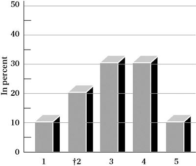
In addition to a table format, frequencies can be visually represented by graphs, such as a pie chart, histogram or bar graph, and polygon (dots connected by lines). Let us use another hypothetical data set to illustrate the value of representing frequencies using some of these formats. Assume you conducted a study with 1000 persons aged 65 years or older in which you obtained scores on a measure of “life satisfaction.” If you examine the raw scores, you will be at a loss to understand patterns or how the group behaves on this measure. One way to begin will be to examine the frequency of scores for each response category of the life satisfaction scale using a histogram. There are five response categories: 5 = very satisfied, 4 = satisfied, 3 = neutral, 2 = unsatisfied, and 1 = very unsatisfied. Figure 19-1 depicts the distribution of the scores by percentage of responses in each category (relative frequency).

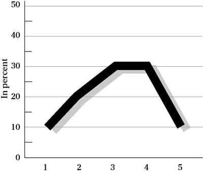
You can also visually represent the same data using a polygon. A dot is plotted for the percentage value, and lines are drawn among the dots to yield a picture of the shape of the distribution, as well as the frequency of responses in each category (Figure 19-2).

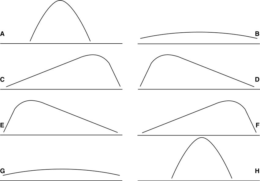
Frequencies can be described by the nature of their distribution. There are several shapes of distributions. Distributions can be symmetrical (Figure 19-3, A and B), in which both halves of the distribution are identical. This distribution is referred to as a normal distribution. Distributions can also be nonsymmetrical (Figure 19-3, C and D) and are characterized as positively or negatively skewed. A distribution that has a positive skew has a curve that is high on the left and a tail to the right (Figure 19-3, E). A distribution that has a negative skew has a curve that is high on the right and a tail to the left (Figure 19-3, F). A distribution can be characterized by its shape, or what is called kurtosis, and is either characterized by its flatness (platykurtic; Figure 19-3, G) or peakedness (leptokurtic; Figure 19-3, H). Not shown is a bimodal distribution, which is characterized by two high points. If you plot the age of the 20 students who registered for the drug prevention course (data shown in Table 19-4), you will have a bimodal distribution.

It is good practice to examine the shape of a distribution before proceeding with other statistical approaches. The shape of the distribution will have important implications for determining central tendency and the other types of analysis that can be performed.

Measures of Central Tendency

A frequency distribution reduces a large collection of data into a relatively compact form. Although we can use terms to describe a frequency distribution (e.g., bell shaped, kurtosis, or skewed to the right), we can also summarize the frequency distribution by using specific numerical values. These values are called measures of central tendency and provide important information regarding the most typical or representative scores in a group. The three basic measures of central tendency are the mode, median, and mean.

Mode

In most data distributions, observations tend to cluster heavily around certain values. One logical measure of central tendency is the value that occurs most frequently. This value is referred to as the “modal value” or the mode. For example, consider the data collection of nine observations, such as the following values:

9 12 15 15 15 16 16 20 26

In this distribution of scores, the modal value is 15 because it occurs more than any other score. The mode therefore represents the actual value of the variable that occurs most often. It does not refer to the frequency associated with that value.

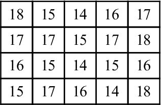
Some distributions can be characterized as “bimodal” in that two values occur with the same frequency. Let us use the age distribution of the 20 students who plan to attend the drug abuse prevention class (see Table 19-4). In this distribution, two categories have the same high frequency. This is a bimodal distribution; 14 is the value of one mode, and 17 is the value of the second mode.

In a distribution based on data that have been grouped into intervals, the mode is often considered to be the numerical midpoint of the interval that contains the highest frequency of observations. For example, let us reexamine the frequency distribution of the students’ ages (see Table 19-5). The first category of ages, 14 to 16 years, represents the highest frequency. However, because the exact ages of the individuals in that category are not known, we select 15 as our mode because it is the midway point of the numerical values contained within this category.

The advantage of the mode is that it can be easily obtained as a single indicator of a large distribution. Also, the mode can be used for statistical procedures with categorical (nominal) variables (numbers assigned to a category; e.g., 15 male and 25 female).

Median

The second measure of central tendency is the median. The median is the point on a scale above or below which 50% of the cases fall. It lies at the midpoint of the distribution. To determine the median, arrange a set of observations from lowest to highest in value. The middle value is singled out so that 50% of the observations fall above and below that value. Consider the following values:

22 24 24 25 27 30 31 35 40

The median is 27, because half the scores fall below the number 27 and half are above. In an odd number of values, as in the previous case of nine, the median is one of the values in the distribution. When an even number of values occurs in a distribution, the median may or may not be one of the actual values, because there is no middle number; in other words, an even number of values exist on both sides of the median. Consider the following values:

22 24 24 25 27 30 31 35 40 47

The median lies between the fifth and sixth values. The median is therefore calculated as an average of the scores surrounding it. In this case, the median is 28.5 because it lies halfway between the values of 27 and 30. If the sixth value had been 27, the median would have been 27. Look at Table 19-4 again. Can you determine the median value? Write out the complete array of ages based on the frequency of their occurrence. For example, age 14 occurs three times, so you list 14 three times; the age of 15 occurs five times, so you list 15 five times; and so forth. Count until the 10th and 11th value. What age did you obtain? If you identified 16, you are correct. The age of 16 years occurs in the 10th and 11th value and is therefore the median value of this group of students.

In the case of a frequency distribution based on grouped data, the median can be reported as the interval in which the cumulative frequency equals 50% (or midpoint of that interval).

The major advantage of the median is that it is insensitive to extreme scores in a distribution; that is, if the highest score in the set of numbers shown had been 85 instead of 47, the median would not be affected. Income is an example of how the median is a good indicator of central tendency because it is not affected by extreme values.

Mean

The mean, as a measure of central tendency, is the most fundamental concept in statistical analysis used with continuous (interval and ratio) data. Remember that different from the mode and median, which do not require mathematical calculations (with the exceptions discussed), the mean is derived from manipulating numbers mathematically. Thus, the data must have the properties that will allow them to be subjected to addition, subtraction, multiplication, and division.

Suppose that you were doing a study in which you were interested in comparing how male and female young adults responded to a smoking prevention program. You assign the number “1” to code male gender and “2” to code female gender. It would not make sense to calculate a mean score for gender because 1 and 2 are nominal and used to identify categories rather than magnitude. Similarly, if you coded ages as 1 = ages 18 to 21, 2 = ages 22 to 25, and 3 = ages 26+, you would not be able to subject your ordinal data (1, 2, 3) to the calculation of the mean because these numbers denote order, not mathematical magnitude.

The mean serves two purposes. First, it serves as a data reduction technique in that it provides a summary value for an entire distribution. Second and equally important, the mean serves as a building block for many other statistical techniques. As such, the mean is of the utmost importance. There are many common symbols for the mean (Box 19-1).

BOX 19-1

Common Symbols for the Mean

Mx = mean of variable x

My = mean of variable y

X¯ = x bar or mean value of a variable

M = mu, mean of a sample

The formula for calculating the mean is simple:

M=ΣXiN

where ΣX_i = sum of all values, M = mean, and N = total number of observations. You may recognize this formula as the one that you learned to calculate averages.

The major advantage of the mean over the mode and median is that in calculating the mean, the numerical value of every observation in the data distribution is considered and used. When the mean is calculated, all values are summed and then divided by the number of values. However, this strength can be a drawback with highly skewed data in which there are outliers or extreme scores, as stated in our discussion of the median. Consider the following example.

Suppose you have just completed teaching a continuing education course in cardiopulmonary resuscitation (CPR). You test your students to determine their competence in CPR knowledge and skill. Of a possible 100, the following scores were obtained:

100 100 100 95 95

To calculate the mean, you will add each value and divide the sum by the total number of values (100 + 100 + 100 + 95 + 95 = 490/5 = 98). The mean score of your group is 98. You are satisfied with the scores and with the high level of knowledge and skill. Now let us see what happens in the following distribution of test scores:

100 100 100 90 35

The mean is calculated as 100 + 100 + 100 + 90 + 35 = 425/5 = 85. The mean (85) presents quite a different picture, even though only one member of the group scored poorly. If only the mean were reported, you would have no way of knowing that the majority of your class did well and that one individual or outlier score was responsible for the lower mean.

Which Measure(s) to Calculate?

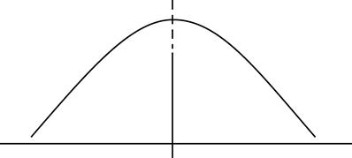
Although investigators often calculate all three measures of central tendency for continuous data, they may not all be useful. Their usefulness depends on the purpose of the analysis and the nature of the distribution of scores. In a normal or bell-shaped curve, the mean, median, and mode are in the same location (Figure 19-4). In this case, it is most efficient to use the mean, because it is the most widely used measure of central tendency and forms the foundation for subsequent statistical calculations.

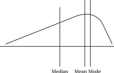
However, in a skewed distribution the three measures of central tendency fall in different places (Figure 19-5). In this case, you will need to examine all three measures and select the one that most reasonably answers your question without providing a misleading picture of the findings.

Now consider another example that illustrates a limitation of the mean. Suppose the scores that were obtained on level of knowledge and skill were:

100 100 100 66 66 66

You calculate the mean as 83 and, because it is close to the mean in the earlier example, surmise that the scores are similar. However, look at the bimodal distribution. What the mean cannot tell you is the shape of the distribution.

Measures of Variability

We have learned that a single numerical index, such as the mean, median, or mode, can be used to describe central tendencies a large frequency of scores but cannot tell you how the scores are distributed. Thus, each measure of central tendency has certain limitations, especially in the case of a distribution with extreme or bimodal scores. Most groups of scores on a scale or index differ from one another, or have what is termed “variability” (also called “spread” or “dispersion”). Variability is another way to summarize and characterize large data sets. By variability, we simply mean the degree of dispersion or the differences among scores. If scores are similar, there is little dispersion, spread, or variability across response categories. However, if scores are dissimilar, there is a high degree of dispersion.

Even though a measure of central tendency provides a numerical index of the average score in a group, as we have illustrated, it is also important to know how the scores vary or how they are dispersed around the measure of central tendency. Measures of variability provide additional information about the scoring patterns of the entire group.

Consider two groups of life satisfaction scores measured as continuous data, as shown in Table 19-6. In both groups, the mean satisfaction score is equal to 100. However, the variability, or dispersion, of scores around the mean is quite different. The scores in Group 1 are more homogeneous. In the second group, the scores are more variable, dispersed, or heterogeneous. The dispersion of scores for the two groups is shown in Figure 19-6. Therefore, knowing the mean will not help ascertain differences in the two groups, even though they exist. Let us assume you had to develop a support-group educational program for both groups. You would approach the focus of each group differently on the basis of your knowledge of the variability in scores.

TABLE 19-6

Life Satisfaction Scores for Two Groups*

Group 1	Group 2
102	128
99	78
103	93
96	101

^*See Figure 19-6.

Only gold members can continue reading. Log In or Register to continue

Share this:

• Click to share on Twitter (Opens in new window)
• Click to share on Facebook (Opens in new window)

Related

Related posts:

1. 11. Setting the Boundaries of a Study
2. 22. Sharing Research Knowledge During and After the Study
3. 7. Formulating Research Questions and Queries
4. 8. Language and Thinking Processes

Stay updated, free articles. Join our Telegram channel

Join