Chapter 11
Understanding Statistics in Research
After completing this chapter, you should be able to:
1. Identify the purposes of statistical analyses.
2. Describe the process of data analysis: (a) management of missing data; (b) description of the sample; (c) reliability of the measurement methods; (d) exploratory analysis of the data; and (e) use of inferential statistical analyses guided by study objectives, questions, or hypotheses.
3. Describe probability theory and decision theory that guide statistical data analysis.
4. Describe the process of inferring from a sample to a population.
5. Discuss the distribution of the normal curve.
6. Compare and contrast type I and type II errors.
7. Identify descriptive analyses, such as frequency distributions, percentages, measures of central tendency, and measures of dispersion, conducted to describe the samples and study variables in research.
8. Describe the results obtained from the inferential statistical analyses conducted to examine relationships (Pearson product-moment correlation and factor analysis) and make predictions (linear and multiple regression analysis).
9. Describe the results obtained from inferential statistical analyses conducted to examine differences, such as chi-square analysis, t-test, analysis of variance, and analysis of covariance.
10. Describe the five types of results obtained from quasi-experimental and experimental studies that are interpreted within a decision theory framework: (a) significant and predicted results; (b) nonsignificant results; (c) significant and unpredicted results; (d) mixed results; and (e) unexpected results.
11. Compare and contrast statistical significance and clinical importance of results.
12. Critically appraise statistical results, findings, limitations, conclusions, generalization of findings, nursing implications, and suggestions for further research in a study.
Analysis of covariance, p. 353
Between-group variance, p. 351
Chi-square test of independence, p. 347
Coefficient of multiple determination, p. 345
Descriptive statistics, p. 319
Frequency distribution, p. 330
Grouped frequency distributions, p. 330
Implications for nursing, p. 356
Inferential statistics, p. 319
Level of statistical significance, p. 325
Measures of central tendency, p. 331
Measures of dispersion, p. 333
Nonparametric analyses, p. 338
Nonsignificant results, p. 353
One-tailed test of significance, p. 327
Paired groups or dependent groups, p. 338
Pearson product-moment correlation, p. 340
Percentage distribution, p. 331
Recommendations for further study, p. 356
Significant and unpredicted results, p. 354
Simple linear regression, p. 344
Statistical techniques, p. 319
Two-tailed test of significance, p. 327
Ungrouped frequency distribution, p. 330
The expectation that nursing practice be based on research evidence has made it important for students and clinical nurses to acquire skills in reading and evaluating the results from statistical analyses (Brown, 2014; Craig & Smyth, 2012). Nurses probably have more anxiety about data analysis and statistical results than they do about any other aspect of the research process. We hope that this chapter will dispel some of that anxiety and facilitate your critical appraisal of research reports. The statistical information in this chapter is provided from the perspective of reading, understanding, and critically appraising the results sections in quantitative studies rather than on selecting statistical procedures for data analysis or performing statistical analyses.
Understanding the Elements of the Statistical Analysis Process
Description of the Sample
Researchers obtain as complete a picture of the sample as possible for their research report. Variables relevant to the sample are called demographic variables and might include age, gender, ethnicity, educational level, and number of chronic illnesses (see Chapter 5). Demographic variables measured at the nominal and ordinal levels, such as gender, ethnicity, and educational level, are analyzed with frequencies and percentages. Estimates of central tendency (e.g., the mean) and dispersion (e.g., the standard deviation) are calculated for variables such as age and number of chronic illnesses that are measured at the ratio level. Analysis of these demographic variables produces the sample characteristics for the study participants or subjects. When a study includes more than one group (e.g., treatment group and control or comparison group), researchers often compare the groups in relation to the demographic variables. For example, it might be important to know whether the groups’ distributions of age and chronic illnesses were similar. When demographic variables are similar for the treatment (intervention) and comparison groups, the study is stronger because the outcomes are more likely to be caused by the intervention rather than by group differences at the start of the study.
 Critical Appraisal Guidelines
Description of the Sample
1. What variables were used to describe the sample?
2. What statistical techniques were used to descriptively analyze the demographic variables, and were these techniques appropriate based on the level of measurement of these variables? Figure 10-2 covers the rules for the nominal, ordinal, interval, and ratio levels of measurement.
3. Was the sample representative of the study target population? For example, was this study’s sample similar to the samples of other studies in this area that were cited in the literature review or the discussion section of the study?
4. If the sample is divided into groups for data analyses, was the similarity or homogeneity of the groups discussed? (See Chapter 9.)
 Research Example
Description of the Sample
Kim, Chung, Park, and Kang (2012) conducted a quasi-experimental study to examine the effectiveness of an aquarobic exercise program on the self-efficacy, pain, body weight, blood lipid levels, and depression of patients with osteoarthritis. The study included 70 subjects, with 35 patients randomly assigned to the experimental group and 35 to the control group. We recommend that you obtain this article, and review this study. The results from this study are presented as examples several times in this chapter to facilitate your understanding of statistical techniques.
The demographic variables used to describe the sample in the Kim and colleagues’ (2012) study included age, educational level, marital status, religion, occupation, income, and health status. Descriptive statistics of frequency and percentage (%) were used to analyze the demographic data, and the experimental and control groups were compared for similarities. The results from these analyses are presented in Table 11-1
Table 11-1
Homogeneity Test of General Characteristics Between Experimental and Control Groups
| Characteristics | Experimental Group | Control Group | p |
| Age (yr) | |||
| 55-59 | 0 (0.0) | 2 (5.7) | 0.545* |
| 60-64 | 11 (31.4) | 9 (25.7) | |
| 65-69 | 15 (42.9) | 17 (48.6) | |
| ≥70 | 9 (25.7) | 7 (20.0) | |
| Educational Level | |||
| None | 4 (11.4) | 1 (2.9) | 0.373* |
| Elementary | 5 (14.3) | 11 (31.4) | |
| Middle school | 15 (42.9) | 14 (40.0) | |
| High school | 5 (14.3) | 5 (14.3) | |
| College or more | 6 (17.1) | 4 (11.4) | |
| Marital Status | |||
| Married | 22 (62.9) | 22 (62.9) | 1.000* |
| Bereavement | 11 (31.4) | 12 (34.3) | |
| Other | 2 (5.7) | 1 (2.9) | |
| Religion | |||
| Christian | 8 (22.9) | 7 (20.0) | 0.907* |
| Catholic | 12 (34.3) | 15 (42.9) | |
| Buddhist | 9 (25.7) | 9 (25.7) | |
| None | 5 (14.3) | 4 (11.4) | |
| Occupation | |||
| Yes | 4 (11.4) | 3 (8.6) | 1.000* |
| None | 31 (88.6) | 32 (91.4) | |
| Income (per/mo) | |||
| <100 | 18 (51.4) | 18 (51.4) | 0.496* |
| 100-200 | 5 (14.3) | 9 (25.7) | |
| 201-300 | 7 (20.0) | 6 (17.1) | |
| >300 | 5 (14.3) | 2 (5.7) | |
| Health Status | |||
| Good | 5 (14.7) | 5 (14.3) | 0.649 |
| Fair | 16 (47.1) | 16 (45.7) | |
| Bad | 13 (38.2) | 14 (40.0) | |
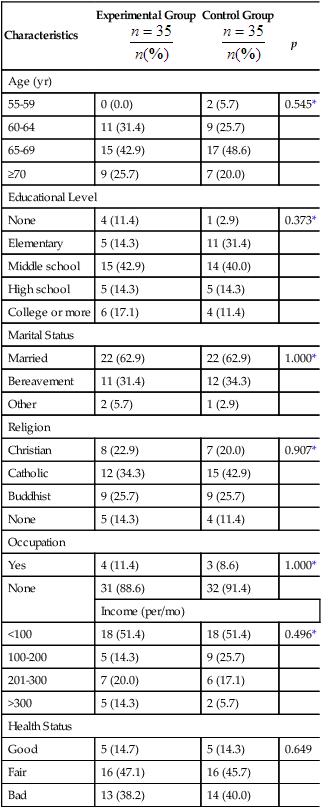
From Kim, I., Chung, S., Park, Y., & Kang, H. (2012). The effectiveness of an aquarobic exercise program for patients with osteoarthritis. Applied Nursing Research, 25(3), p. 186 (Table 2 from the article).
Kim and associates (2012) developed a table that clearly presented the results of their analysis of demographic variables, and they discussed this table in the results section of their research report. The demographic variables of age, educational level, marital status, occupation, and income are commonly used in many studies to describe the samples. The descriptive analysis techniques of frequency and percentage were appropriate for the demographic variables measured at the nominal or ordinal level. Age, educational level, income, and health status were measured at the ordinal level, and marital status, religion, and occupation were measured at the nominal level.
Kim and co-workers (2012) implemented a structured aquarobic exercise program that included two educational sessions, followed by selected aerobic exercises. The aquarobic exercises are detailed in a table in the article and involved an instructor leading the patients with osteoarthritis through various aerobic exercises in the water for 1 hour, three times a week, for a total of 36 sessions over 12 weeks. The researchers found that the “Aquarobic Exercise Program was effective in enhancing self-efficacy, decreasing pain, and improving depression levels, body weight, and blood lipid levels in patients with osteoarthritis” (Kim et al., 2012, p. 181). They recommended the use of this program in managing patients with osteoarthritis but also recognized the need for additional research to determine the long-term benefits of this program for these patients. The Quality and Safety Education for Nursing Institute (QSEN, 2013) provides competencies for prelicensure nurses. The QSEN implication of this research report is the evidence-based intervention of an aquarobic exercise program, which improved the health outcomes for these patients with osteoarthritis. Nurses and students are encouraged to use research findings in promoting an evidence-based practice (EBP) for nursing.
Reliability of Measurement Methods
Researchers need to report the reliability of the measurement methods used in their study. The reliability of observational or physiological measures is usually determined during the data collection phase and needs to be noted in the research report. If a scale was used to collect data, the Cronbach alpha procedure needs to be applied to the scale items to determine the reliability of the scale for this study (Waltz, Strickland, & Lenz, 2010). If the Cronbach alpha coefficient is unacceptably low (< 0.70), the researcher must decide whether to analyze the data collected with the instrument. A value of 0.70 is considered acceptable, especially for newly developed scales. A Cronbach alpha coefficient value of 0.80 to 0.89 from previous research indicates that a scale is sufficiently reliable to use in a study (see Chapter 10). The t-test or Pearson’s correlation statistics may be used to determine test-retest reliability (Grove, Burns, & Gray, 2013). In critically appraising a study, you need to examine the reliability of the measurement methods and the statistical procedures used to determine these values. Sometimes researchers examine the validity of the measurement methods used in their studies, and this content also needs to be included in the research report (see Chapter 10).
An example is presented from the Kim and colleagues’ (2012) study (see earlier). They measured self-efficacy with a 14-item Likert-type scale that had been previously developed for patients with arthritis. The higher scores indicated greater levels of self-efficacy. The calculated Cronbach alpha for this scale in this study was 0.90, indicating 90% reliability or consistency in the measurement of self-efficacy and 10% error. Kim and associates (2012) measured depression with the Zung Self-Rating Depression Scale, which “consisted of 20 items (10 positive and 10 negative) on a 4-point Likert-type scale. Negative responses were converted into scores, and higher scores indicated greater levels of depression. Cronbach’s alpha in this study was 0.75” (75% reliability and 25% error; Kim et al., 2012, p. 185). This study included a concise description of the scales used to collect psychosocial data and documented the scales’ reliability using Cronbach alpha values. The reliability of the self-efficacy scale was strong at 0.90, but the Zung Self-Rating Depression Scale reliability (0.75) was a little low for an established scale.
Inferential Statistical Analyses
The final phase of data analysis involves conducting inferential statistical analyses for the purpose of generalizing findings from the study sample to appropriate accessible and target populations. To justify generalization of the results from inferential statistical analyses, a rigorous research methodology is needed, including a strong research design (Shadish, Cook, Campbell, 2002), reliable and valid measurement methods (Waltz et al., 2010), and a large sample size (Cohen, 1988).
Most researchers include a section in their research report that identifies the statistical analysis techniques conducted on the study data and the program used to calculate them. This discussion includes the inferential analysis techniques (e.g., those focused on relationships, prediction, and differences) and sometimes the descriptive analysis techniques (e.g., frequencies, percentages, and measures of central tendency and dispersion) conducted in the study. The identification of data analysis techniques conducted in a study are usually presented just prior to the study’s results section. Kim and co-workers (2012) had a strong pretest and post-test quasi-experimental design with experimental and control groups (see Chapter 8). The study variables were measured with fairly reliable scales and accurate and precise physiological instruments. The inferential statistical analyses conducted were clearly identified and focused on addressing the study purpose. This study excerpt identifies the analysis techniques:
“Data Analysis
Data analysis was performed using SPSS [Statistical Package for the Social Sciences] version 12.0. Homogeneity of the two groups was assessed using Fisher’s exact test, the chi-square test, and independent t-tests [discussed later in this chapter]. Comparisons of posttest values for the experimental and control groups were then made using independent t-tests.” (Kim et al., 2012, p. 185)
Understanding Theories and Concepts of the Statistical Analysis Process
This section presents a brief explanation of some of the theories and concepts important in understanding the statistical analysis process. Probability theory and decision theory are discussed, and the concepts of hypothesis testing, level of significance, inference, generalization, the normal curve, tailedness, type I and type II errors, power, and degrees of freedom are described. More extensive discussion of these topics can be found in other sources, and we recommend our own textbooks (Grove, 2007; Grove et al., 2013) and a quality statistical text by Plichta and Kelvin (2013).
Decision Theory, Hypothesis Testing, and Level of Significance
Decision theory assumes that all of the groups in a study (e.g., experimental and comparison groups) used to test a particular hypothesis are components of the same population relative to the variables under study. This expectation (or assumption) traditionally is expressed as a null hypothesis, which states that there is no difference between (or among) the groups in a study, in terms of the variables included in the hypothesis (see Chapter 5 for more details of types of hypotheses). It is up to the researcher to provide evidence for a genuine difference between the groups. For example, the researcher may hypothesize that the frequency of UTIs that occurred after discharge from the hospital in patients who were catheterized during hospitalization is no different from the frequency of such infections in those who were not catheterized. To test the assumption of no difference, a cutoff point is selected before data collection. The cutoff point, referred to as alpha (α), or the level of statistical significance, is the probability level at which the results of statistical analysis are judged to indicate a statistically significant difference between the groups. The level of significance selected for most nursing studies is 0.05. If the p value found in the statistical analysis is less than or equal to 0.05, the experimental and comparison groups are considered to be significantly different (members of different populations).
Decision theory requires that the cutoff point selected for a study be absolute. Absolute means that even if the value obtained is only a fraction above the cutoff point, the samples are considered to be from the same population, and no meaning can be attributed to the differences. It is inappropriate when using decision theory to state that the findings approached significance at p = 0.051 if the alpha level was set at 0.05. Using decision theory rules, this finding indicates that the groups tested are not significantly different, and the null hypothesis is accepted. On the other hand, once the level of significance has been set at 0.05 by the researcher, if the analysis reveals a significant difference of 0.001, this result is not considered more significant than the 0.05 originally proposed (Slakter, Wu, & Suzaki-Slakter, 1991). The level of significance is dichotomous, which means that the difference is significant or not significant; there are no “degrees” of significance. However, some people, not realizing that their reasoning has shifted from decision theory to probability theory, indicate in their research report that the 0.001 result makes the findings more significant than if they had obtained only a 0.05 level of significance.
Normal Curve
A normal curve is a theoretical frequency distribution of all possible values in a population; however, no real distribution exactly fits the normal curve (Figure 11-1). The idea of the normal curve was developed by an 18-year-old mathematician, Johann Gauss, in 1795. He found that data from variables (e.g., the mean of each sample) measured repeatedly in many samples from the same population can be combined into one large sample. From this large sample, a more accurate representation can be developed of the pattern of the curve in that population than is possible with only one sample. Surprisingly, in most cases, the curve is similar, regardless of the specific variables examined or the population studied.
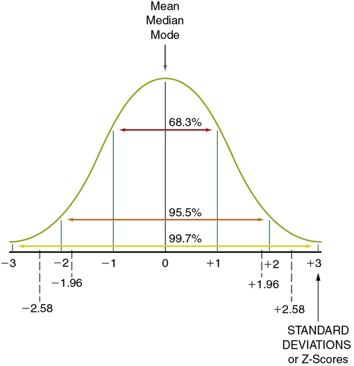
Levels of significance and probability are based on the logic of the normal curve. The normal curve presented in Figure 11-1 shows the distribution of values for a single population. Note that 95.5% of the values are within 2 standard deviations (SDs) of the mean, ranging from − 2 to + 2 SDs. (Standard deviation is described later in this chapter; see “Using Statistics to Describe.”) Thus there is approximately a 95% probability that a given measured value (e.g., the mean of a group) would fall within approximately 2 SDs of the mean of the population, and there is a 5% probability that the value would fall in the tails of the normal curve (the extreme ends of the normal curve, below − 2 (− 1.96 exactly) SDs [2.5%] or above + 2 (+ 1.96 exactly) SDs [2.5%]). If the groups being compared are from the same population (not significantly different), you would expect the values (e.g., the means) of each group to fall within the 95% range of values on the normal curve. If the groups are from (significantly) different populations, you would expect one of the group values to be outside the 95% range of values. An inferential statistical analysis performed to determine differences between groups, using a level of significance (α) set at 0.05, would test that expectation. If the statistical test demonstrates a significant difference (the value of one group does not fall within the 95% range of values), the groups are considered to belong to different populations. However, in 5% of statistical tests, the value of one of the groups can be expected to fall outside the 95% range of values but still belong to the same population (a type I error).
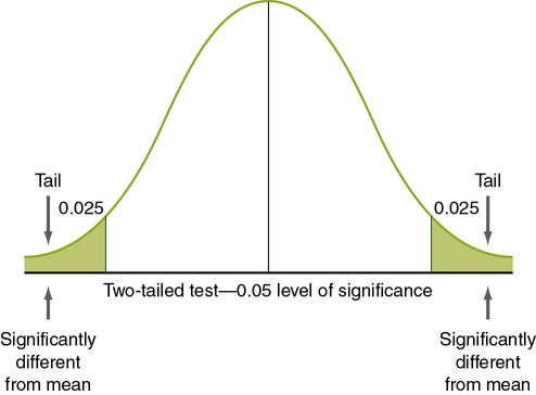
Tailedness
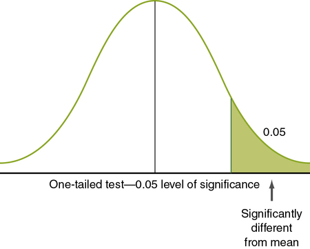
Nondirectional hypotheses usually assume that an extreme score (obtained because the group with the extreme score did not belong to the same population) can occur in either tail of the normal curve (Figure 11-2). The analysis of a nondirectional hypothesis is called a two-tailed test of significance. In a one-tailed test of significance, the hypothesis is directional, and extreme statistical values that occur in a single tail of the curve are of interest (see Chapter 5 for a discussion of directional and nondirectional hypotheses). The hypothesis states that the extreme score is higher or lower than that for 95% of the population, indicating that the sample with the extreme score is not a member of the same population. In this case, 5% of statistical values that are considered significant will be in one tail, rather than two. Extreme statistical values occurring in the other tail of the curve are not considered significantly different. In Figure 11-3, which shows a one-tailed figure, the portion of the curve in which statistical values will be considered significant is the right tail. Developing a one-tailed hypothesis requires that the researcher have sufficient knowledge of the variables to predict whether the difference will be in the tail above the mean or in the tail below the mean. One-tailed statistical tests are uniformly more powerful than two-tailed tests, decreasing the possibility of a type II error (saying something is not significant when it is).
Type I and Type II Errors
According to decision theory, two types of error can occur when a researcher is deciding what the result of a statistical test means, type I and type II (Table 11-2). A type I error occurs when the null hypothesis is rejected when it is true (e.g., when the results indicate that there is a significant difference, when in reality there is not). The risk of a type I error is indicated by the level of significance. There is a greater risk of a type I error with a 0.05 level of significance (5 chances for error in 100) than with a 0.01 level of significance (1 chance for error in 100).
Table 11-2
| In Reality, The Null Hypothesis* Is: | ||
| Data Analysis Indicates | True | False |
| Results significant, null hypothesis rejected | Type I error (α) | Correct decision (power) |
| Results not significant, null hypothesis not rejected | Correct decision | Type II error (β) |
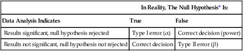
*The null hypothesis is stating that no difference or relationship exists.
A type II error occurs when the null hypothesis is regarded as true but is in fact false. For example, statistical analyses may indicate no significant differences between groups, but in reality the groups are different (see Table 11-2). There is a greater risk of a type II error when the level of significance is 0.01 than when it is 0.05. However, type II errors are often caused by flaws in the research methods. In nursing research, many studies are conducted with small samples and with instruments that do not accurately and precisely measure the variables under study (Grove et al., 2013; Waltz et al., 2010). In many nursing situations, multiple variables interact to cause differences within populations. When only a few of the interacting variables are examined, small differences between groups may be overlooked. This leads to nonsignificant study results, which can cause researchers to conclude falsely that there are no differences between the samples when there actually are. Thus the risk of a type II error is often high in nursing studies.
Power: Controlling the Risk of a Type II Error
Power is the probability that a statistical test will detect a significant difference that exists (see Table 11-2). The risk of a type II error can be determined using power analysis. Cohen (1988) has identified four parameters of a power analysis: (1) the level of significance; (2) sample size; (3) power; and (4) effect size. If three of the four are known, the fourth can be calculated using power analysis formulas. The minimum acceptable power level is 0.80 (80%). The researcher determines the sample size and the level of significance (usually set at α = 0.05). (Chapter 9 provides a detailed discussion of power analysis.) Effect size is “the degree to which the phenomenon is present in the population, or the degree to which the null hypothesis is false” (Cohen, 1988, pp. 9-10). For example, if changes in anxiety level are measured in a group of patients before surgery, with the first measurement taken when the patients are still at home, and the second taken just before surgery, the effect size will be large if a great change in anxiety occurs in the group between the two points in time. If the effect of a preoperative teaching program on the level of anxiety is measured, the effect size will be the difference in the post-test level of anxiety in the experimental group compared with that in the comparison group. If only a small change in the level of anxiety is expected, the effect size will be small. In many nursing studies, only small effect sizes can be expected. In such a study, a sample of 200 or more is often needed to detect a significant difference (Cohen, 1988). Small effect sizes occur in nursing studies with small samples, weak study designs, and measurement methods that measure only large changes. The power level should be discussed in studies that fail to reject the null hypothesis (or have nonsignificant findings). If the power level is below 0.80, you need to question the validity of the nonsignificant findings.
Degrees of Freedom
The concept of degrees of freedom (df) is important for calculating statistical procedures and interpreting the results using statistical tables. Degrees of freedom involve the freedom of a score value to vary given the other existing scores’ values and the established sum of these scores (Grove et al., 2013). Degrees of freedom are often reported with statistical results.
Using Statistics to Describe
Frequency Distributions
Ungrouped Frequency Distributions
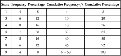
Most studies have some categorical data that are presented in the form of an ungrouped frequency distribution, in which a table is developed to display all numerical values obtained for a particular variable. This approach is generally used on discrete rather than continuous data. Examples of data commonly organized in this manner are gender, ethnicity, marital status, diagnoses of study subjects, and values obtained from the measurement of selected research and dependent variables. Table 11-3 is an example table developed for this text; it includes nine different scores obtained by 50 subjects. This is an example of ungrouped frequencies because each score is represented in the table with the number of subjects receiving this score.
Table 11-3
Example of an Ungrouped Frequency Table
| Score | Frequency | Percentage | Cumulative Frequency (f) | Cumulative Percentage |
| 1 | 4 | 8 | 4 | 8 |
| 3 | 6 | 12 | 10 | 20 |
| 4 | 8 | 16 | 18 | 36 |
| 5 | 14 | 28 | 32 | 64 |
| 7 | 8 | 16 | 40 | 80 |
| 8 | 6 | 12 | 46 | 92 |
| 9 | 4 | 8 | N = 50 | 100 |
Grouped Frequency Distributions
Grouped frequency distributions are used when continuous variables are being examined. Many measures taken during data collection, including body temperature, vital lung capacity, weight, age, scale scores, and time, are measured using a continuous scale. Any method of grouping results in loss of information. For example, if age is grouped, a breakdown into two groups, younger than 65 years and older than 65 years, provides less information about the data than groupings of 10-year age spans. As with levels of measurement, rules have been established to guide classification systems. There should be at least five but not more than 20 groups. The classes established must be exhaustive; each datum must fit into one of the identified classes. The classes must be exclusive; each datum must fit into only one (Grove et al., 2013). A common mistake occurs when the ranges contain overlaps that would allow a datum to fit into more than one class. For example, a researcher may classify age ranges as 20 to 30, 30 to 40, 40 to 50, and so on. By this definition, subjects aged 30, 40, and so on can be classified into more than one category. The range of each category must be equivalent. For example, if 10 years is the age range, each age category must include 10 years of ages. This rule is violated in some cases to allow the first and last categories to be open-ended and worded to include all scores above or below a specified point. Table 11-4 is an example of a grouped frequency distribution for income for registered nurses (RNs), in which the categories are exhaustive and mutually exclusive.
Table 11-4
Income of Full-Time Registered Nurses (n = 100)
| Income | Frequency (%) |
| Below $60,000 | 5 (5%) |
| $60,000-69,999 | 20 (20%) |
| $70,000-79,999 | 35 (35%) |
| $80,000-90,000 | 25 (25%) |
| Above $90,000 | 15 (15%) |
Stay updated, free articles. Join our Telegram channel

Full access? Get Clinical Tree


