Introduction
This chapter is linked to the analysing data section of the web program.
As well as describing how you intend collecting the data for your research study in your research proposal, you need to state how you will analyse the data. The problem is that ‘raw’ data on their own are meaningless, so before we can use the data, they need to be organised and interpreted – in other words, analysed (Botti & Endacott 2005).
If you have data from a quantitative research study, they will normally be in a numerical form; in order to use these data, you need to use statistics to analyse them. For many people, the term statistics can immediately make them panic, even mentally switch off, but in fact dealing with statistics can be fun! We all use statistics every day without thinking of it as statistics. The statistics we typically use most frequently are ‘averages’ and ‘percentages’ – as in the average age of the footballers playing for Manchester City is …, or the percentage of girls who go to university to take a nursing degree is …,and so on. So statistics are nothing to fret about, as you will discover as you work through this chapter.
Totally different from the analysis of data obtained from a quantitative research study is the analysis of data obtained from a qualitative research study. Here the data may be numerical, but they mainly comprise words, or sometimes non-verbal and non-numerical data such as drawings. In many ways, qualitative research data are harder to analyse because, unlike with quantitative research data which convert readily to statistics – and there are many different tests/computer programs to analyse the statistics for you – qualitative data analysis is less direct and possibly a little nebulous, as you will see. Although there are certain processes that we can use to help us analyse our qualitative data, the fact is that qualitative data are more open to interpretation than are quantitative data. Therefore, we shall start by looking at, and discussing, how we can analyse data from quantitative research studies.
Quantitative data analysis
First, a brief resume of the types of data collection from chapter 8.
When we are undertaking quantitative research, data collection involves the production of numerical data to address the research objectives, questions and/or hypotheses. During this process, the variables in the study are measured using a variety of techniques, including:
- observation;
- interview;
- questionnaire;
- scales;
- physiological measurements.
Data analysis
What do we mean by data analysis? Well, data analysis is a process we use in order to reduce, organise and give meaning to the data we have collected by using the data collection tools discussed in chapter 8. Within quantitative research, the analysis of data involves the use of:
- descriptive and exploratory procedures to describe the study variables and the sample;
- statistical techniques in order to test any proposed relationships;
- techniques that will help us to make predictions;
- techniques that will allow us to examine cause and effect.
It is worth pointing out at that, unlike in the past, when dealing with statistics we no longer need to do calculations ourselves. Computers can perform most analyses.
The choice of technique that is used in any research study is determined mainly by:
- the research objectives, questions or hypotheses;
- the research design;
- the research instruments and how/what they can measure.
So, without further ado, let us start by looking at how we can undertake and analyse quantitative research, with a brief introduction to statistics.
Introduction to statistics
Always treat statistics with caution as well as respect, for as the British prime minister Benjamin Disraeli (1804–1881) once famously (or infamously) said: ‘There are three kinds of lies: lies, damned lies and statistics.’
In this section we are going to take a general look at what we mean by statistics and statistical data. So, let us start with some definitions:
Data
We talk about data in statistics. Data (singular ‘datum’) are things known or assumed as a basis for inference, or, to put it more simply, ‘Pieces of information that are collected during a study’ (Burns & Grove 2005: 733).
Statistics
Statistics are concerned with the systematic collection of numerical data and their interpretation. Burns & Grove (2005: 752) refer to a statistic as simply ‘a numerical value obtained from a sample that is used to estimate the parameters of a population’ . The word’statistics’ can be used to refer to:
- numerical facts, such as the number of people living in a particular town;
- the study of ways of collecting and interpreting these facts.
It can be argued that figures are not facts in themselves. It is only when they are interpreted that they become relevant to discussions and decisions. So statistics are there to inform our discussions – they are a means to an end, not an end in themselves.
Sample
You may recall from chapter 7 that a sample is a group of people, events, behaviours or other elements you need to have in order to conduct your research study.
Population
A population is what we call the group of individuals or elements that meets the sampling criteria (a sample being representative of that population). So, if we were interested in looking at the number of childhood cancers diagnosed in 2006 in the United Kingdom (i.e. our ‘population’), we might not be able to survey the entire population of children with cancer in that year living in the UK, and so we would look at a sample taken from all the children with cancer in 2006 living in the UK (see chapter 7 for the criteria we need to apply to our sample).
Parameter
Parameter has, like many English words, several meanings. According to the Concise Oxford Dictionary (1991) it can be defined as:
- a quantity constant in the case considered but varying in different cases;
- a measurable (or quantifiable) characteristic or feature;
- a constant element or factor, particularly serving as a limit or boundary.
You may be wondering at this point what this means in terms of research. Well, to simplify matters, let us look at the definition given by Burns & Grove (2005 : 745): ‘a measure or numerical value of a population’ – in other words, the numbers found in any given population.
Statistics can be divided into two types:
Descriptive statistics
Description ‘involves identifying and understanding the nature and attributes of nursing phenomena and sometimes the relationships among these phenomena’ (Burns & Grove 2005: 733). According to Sim & Wright (2000), descriptive statistics have two functions:
Descriptive statistics include the presentation of data in tables and diagrams, as well as the calculation of percentages, averages, measures of dispersion (the variation or variability within the statistics) and correlation (the degree of relationship between two variables), in order to show the relevant features of the data and reduce them to manageable proportions. In other words, descriptive statistics involve the summary of the statistics in such a way that the researcher can organise the data in these statistics and give them meaning and insight.
Inductive/inferential statistics
Inductive or inferential statistics involve methods of inferring properties of a population on the basis of known results from a sample that is representative of the population.
To infer is to deduce or conclude from facts and reasoning (Shorter Oxford English Dictionary 2007), and inference is the use of inductive reasoning to move from a specific case to a general truth (and hence is also known as inductive reasoning). The Shorter Oxford English Dictionary gives one meaning of inductive as ‘leading on to’, and according to Burns & Grove (2005: 739), in relation to statistics, inductive reasoning is ‘reasoning from the specific to the general in which particular instances are observed and then combined into a larger whole – or general statement’.
Thus, with these types of statistics, statistics are used to infer results from the specific study of a sample to a general statement about the larger population. So, inferential statistics are statistics that are designed to allow an inference to be made from a sample statistic to a population parameter. They are commonly used to test hypotheses (see chapter 5) that consist of similarities and differences in subsets of the sample under study.
These methods are based directly on probability theory. Probability theory ‘addresses relative rather than absolute causality. Thus, from a probability perspective, a cause will not produce a specific effect each time that particular cause occurs, but the probability value indicates how frequently the effect might occur with the cause’ (Burns & Grove 2005: 747); in other words, given a certain situation, behaviour or event, how often that situation, behaviour or event might cause a particular result.
So much for the general background to statistics; now we can start to look at some actual simple statistics. To begin with, you need to know that symbols are used in statistics to simplify their presentation. Some of the more common ones are given below.
- μ (lower-case Greek letter mu) = the mean
- χ (lower-case Greek letter chi) = each of the individual operations
- Σ (capital Greek letter sigma) = the operation of summing all the values of χ.
- n = number of observations
- σ (lower-case Greek letter sigma) = standard deviation (also symbolised by ‘s’).
- x = mean value
- s2 = variance
- SS = sum of squared errors
When you come to the statistical equations, you can refer to this list for the meanings of the symbols. Now, to boost your confidence and to demonstrate that statistics can be quite simple (and perhaps a little fun) it is time to look at some simple and common statistical calculations, which are regularly used in statistics – and to some extent in our everyday lives, although you may not be aware that you are using them.
Average
‘Average’ is a measure of central tendency and of location. It summarises a group of figures and smoothes out any abnormalities. It also provides a mental picture of the distribution that it represents. In addition, it can provide knowledge about the whole distribution. The word is often used loosely in everyday conversation; however, used in this way, it can conceal important facts.
There is more than one kind of average, so we shall consider these next, commencing with the type that we use most often when we talk about the ‘average’.
Arithmetic mean
‘Arithmetic mean’ is the type of average to which most people refer when they use the word ‘average’, and it can be defined as the sum of the items divided by the number of these items. So,
arithmetic mean = ‘the total value of items’ % the ‘total number of items’
or in symbols:
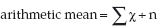
Where Σ = the sum of χ (value of items) and n = number of items.

For example, if we were to look at the ages of child branch student nurses, a group of 21 students, in their first year the university, we might find that there are:
- 11 aged 18 years
- 5 aged 19
- 2 aged 20
- 1 aged 25
- 1 aged 33
- 1 aged 51
According to our equation, to get the arithmetic mean of the group’ s age, we add all the ages together (= 442) and divide that by 21. This gives us an average of 21 years (or 21.047619 if you used a calculator).
So we can see that the average age of this group of students on commencement at the university is 21 years. But can we now say that the age of child branch students on commencing university everywhere is 21 years? Hopefully, your answer is no. After what you have read in chapter 7 and 8, as well as in the web program, you should have realised that the group (our sample) is far too small for us to be able to generalise to child branch students everywhere else (the population).
You should also have noticed that, even in our small sample, our average of 21 years conceals a very important fact: the great majority of these students are aged 18–20 years when they commence university; there are just three students in the group who are aged 21 years or over. Therefore, the average does not give an accurate idea of the group’s age range, let alone allowing us to generalise. Always bear in mind the words of Thomas Carlyle (1840: 9) ‘A witty statesman said, you might prove anything by figures.’
However, we do have a couple of calculations that we can do with these figures that can give us a more realistic average. The first of these is the median.
Median
The median, another type of average, is the value of the middle item of a distribution which is set out in order.
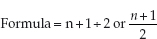
i.e. n plus 1 divided by 2, where n is the number of items.
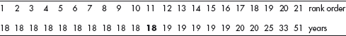
Now we can return to the ages of the cohort of 21 child branch student nurses when they commence at the university, namely:
- 11 aged 18 years
- 5 aged 19
- 2 aged 20
- 1 aged 25
- 1 aged 33
- 1 aged 51
Did you get the same answer?
You can see that the mid-point is the age at rank order number 11, which in this case is 18 years (as there are ten ages before that one and ten after it).
If we look at the formula  , then the mid-point is 21+1 divided
by 2, or 
i.e. in this case the eleventh age in the row, which is 18.
In our example, does the median age give a more accurate idea of the group as a whole than the arithmetic mean average does? I think you would agree that the answer has to be yes, because 18 years is closer to the age of the great majority of the group. However, it still does not identify the anomaly that is the ages of the older students.
So, we have yet another type of average to look at – the mode.
Mode
The mode is the numerical value of a score that occurs with the greatest frequency in a distribution. However, it does not necessarily indicate the centre of the set of data (Burns & Grove 2005).
Again, use the ages to work out the mode (remember that the mode is the number that occurs most often):
- 11 aged 18 years
- 5 aged 19
- 2 aged 20
- 1 aged 25
- 1 aged 33
- 1 aged 51
In this case, 18 years of age occurs more frequently than any other age in our group; therefore the mode of the group is 18 years.
In this case, the mode is the same as the median (but both are different from the mean), but this is not always the case. Consequently, you need to look closely at any statistics, because they are not always what they seem to be.
Finally, let us look at range.
Range
The range is an everyday method of describing the dispersion (spread) of data. It can be defined as the highest value in a distribution less the lowest. Let us look again at our group of child branch student nurses. The range of ages is 18–51 years. Therefore, the range of ages is 51 – 18 years = 33 years. If you combine this with a modal age of 18, what does this tell you about the general age of student nurses in the child branch?
Answer: with a modal age of 18, although there is a range of 33 years (from 18 to 51 years), whilst most of the student nurses are young, there are some older ones (and even one of 51 years), but most of the child branch student nurses are at the younger end of the age range.
So, you can see that statistics are not just a string of numbers and lots of calculations, but are a starting point for debate and discussion.
Reflection on averages
Often range is given along with mean, median or mode. Why?
Answer: the advantage of giving range and one of the averages is that you get a much better idea of the group’s ages as in the example of the child branch student nurses. It also overcomes the problem of how we demonstrate that there are some major anomalies in our group, which are virtually ignored by the various averages. (The ‘anomalies’ in our example are the students who are much older than most of the group.)
So, we can say that the group of child branch student nurses has a:
- mean of 21 years
- median of 18 years
- mode of 18 years
- range of 18–51 years
and we now have a clearer picture of the group in terms of their ages.
Standard deviation
We just have one more important simple statistic to discuss: standard deviation.
Standard deviation is a simple measure of the variability or dispersion (distribution) of a set of data. Basically, it measures the spread of the data about the mean value. A low standard deviation is an indication that all the individual data points are very close to the same value (i.e. the mean – see above), while a high standard deviation is an indication that the data are spread over a wide range of values.
There is a formula to help us to work out standard deviation:
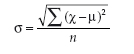
The same symbol you were introduced to earlier are relevant to this formula. So this formula (in words) is ‘Standard deviation (σ) equals the square root (√) of the sum of (Σ) the mean value minus the mean squared ([χ–μ]2), divided by the number of observations (n).
For an example of how we calculate a standard deviation, let us look at the group of students (our population) we used above in our discussion of averages.
We want to find the standard deviation of:
18 18 18 18 18 18 18 18 18 18 18 19 19 19 19 19 20 20 25 33 51 years
First, we have to work out the arithmetic mean. We have already done this and obtained a mean of 21. Now we need to subtract that from each of the ages and square the result. So, for example, 18 – 21 = –3, and squared = 9 (minus numbers squared = positive numbers).
| Score | Deviation | Squared deviation |
| χ | χ − μ | (χ − μ)2 |
| 18 | −3 | 9 |
| 18 | −3 | 9 |
| 18 | −3 | 9 |
| 18 | −3 | 9 |
| 18 | −3 | 9 |
| 18 | −3 | 9 |
| 18 | −3 | 9 |
| 18 | −3 | 9 |
| 18 | −3 | 9 |
| 18 | −3 | 9 |
| 18 | −3 | 9 |
| 19 | −2 | 4 |
| 19 | −2 | 4 |
| 19 | −2 | 4 |
| 19 | −2 | 4 |
| 19 | −2 | 4 |
| 20 | −1 | 2 |
| 20 | −1 | 2 |
| 25 | 4 | 16 |
| 33 | 12 | 144 |
| 51 | 12 | 900 |
Next we have to add up these results. (This is where a calculator comes in handy, and even more so for the next two parts of the equation.)
The total of the squared deviations is 1,183, which we now divide by the number of subjects (21), or 1,183 ÷ 21 = 56.34. Now find the square root of 56.34, which is 7.505997601918082 (rounded = 7.5).
This is the standard deviation, but what do we do with it? The 7.5 score that we have for this group of students is used to give us an idea of the spread of the data that we have regarding the age of the age range.
So if the mean is 21, first we have to see how many of the students fall within one standard deviation (i.e. 7.5) of the mean. In other words, how many students fall within the range of 13.5 – 28.5 (7.5 either side of 21). Well, 18 out of 21 fall between 13.5 and 21, whilst one falls within the range between 21 and 28.5. That means that 19 out of 21 (90%) of the student nurses fall within one standard deviation of the mean. Next we look at how many fall between 6 and 13.5 and between 28.5 and 36 (i.e. within the second standard deviation). The answer is that none falls between 6 and 13.5, and one falls between 28.5 and 36 (5%). Finally, three standard deviations would be ages between 0 and 6 and between 36 and 43.5 – the answer is none. The only remaining student falls between 43.5 and 51, which is four standard deviations. So, given these results, it is clear that, although the group is very homogeneous as regards their ages, there are two students who cause the spread of data to be extensive. According to Hinton (1995: 15–16), in many cases ‘most of the scores (about two-thirds – about 66.7%) will lie within one standard deviation less than, and one standard deviation greater than, the mean’. Our group does not quite fit that finding, with 90% being within one standard deviation, however, there is a special reason for this, and that is that our population is unique in that student nurses, particularly child branch students, are generally starting out in the world afterleaving school, and so they will generally be around the same age.
A word of caution – the formula works for a population. If, however,we wanted to calculate the standard deviation of a sample, the formula is slightly different, namely:

However, the rest of the calculation is as described above, but with the final stage of the calculation using the denominator n – 1 rather than just n.
Summary
This concludes our brief look at statistics. All the statistics you will encounter are variants of these. Some of them may be more complicated, but, like the examples given above, all are attempting to make sense of numerical data.
Finally, a reminder to be wary of statistics when they are presented to you:
‘He uses statistics as a drunken man uses a lamp post – for support rather than illumination’ (attributed to Andrew Lang, 1844–1912) .
Data analysis
Let us commence our look at data analysis by looking at a hypothetical research study.
There are different ways of approaching our research question/ hypothesis, and the way we put together our research question will determine the type of methodology, data collection method, statistics, analysis and presentation we shall use to approach our research problem.
Examples of research questions
- Are females more likely to be nurses than males?
- Is the proportion of males who are nurses the same as the proportion of females?
- Is there a relationship between gender and becoming a nurse?
In these examples, you can see that there are three ways to approach the research problem, which is concerned with the relationship between males and females in nursing, but the way in which the problem is expressed as a question will determine your methodology.
Another research problem with variables


