Chapter 35. Inferential Statistics
Roger Watson
▪ What is inferential statistics?
▪ Confidence
▪ Statistical significance
▪ Differences between means
▪ Correlation
▪ How many subjects?
▪ Conclusion
What is inferential statistics?
Inferential statistics is concerned with applying conclusions to something wider than the observation at hand due to some properties of that observation. For example, if we met a group of people – men and women – and the women earned more than the men, we could infer that women, generally, earned more than men. What inferential statistics allows us to do is make that inference (or not) with some degree of certainty that what we are inferring from the sample applies to a wider group of men and women, i.e. the population of men and women (Swinscow & Campbell 2002).
Confidence
One of the first concepts to understand in inferential statistics is that of confidence, which means the confidence with which we can make an inference about a population based on a sample (Gardner & Altman 2000). For example, if we wished to study the patients on a medical ward, all of whom were admitted with a diagnosis of either heart disease or another diagnosis, and to find out how many of each there were, then this can be used to illustrate confidence. In a ward with a limited number of beds we can easily check the patient records or ask the nurse in charge and we will have an answer. However, suppose that you wish to know how many people in the general population with a medical diagnosis have either heart disease or another diagnosis, then we cannot simply ask someone to check all their records – there are too many of them to make this practical. If we consider all the patients on our ward to be the population and there are 20 beds on the ward, then we can start by finding out the diagnosis of one patient; if this patient’s diagnosis is not heart disease then we know that the number of patients with heart disease lies between 0 and 19. If we find out the diagnosis of a second patient is heart disease then we know, with a greater degree of confidence, that the number of patients with heart disease lies between one and 18. The more patients whose diagnosis we discover, the nearer we get to the true figure for those with heart disease until we sample them all. In reality, it is very rare to be able to obtain the whole population for any study; we almost always work with samples and inferential statistics is concerned with drawing conclusions about the population based on a sample.
Confidence intervals
The example above, where we considered the concept of confidence, leads us naturally to the first concept in inferential statistics: the confidence interval. A confidence interval is a range of values between which a population statistic is thought to lie, with a particular degree – usually 95% – of confidence (Watson et al 2006).
Taking the example of a mean value for a population parameter, for example height, we can take a sample and, as described in the previous chapter, calculate a mean for the sample. We can also calculate a standard deviation of the mean for that sample, the standard deviation being a measure of the spread of the data. The standard deviation is related to the normal distribution, mentioned in the previous chapter, and describes a set proportion of the sample. One standard deviation either side of the mean includes 68% of the sample; two standard deviations 95% and three standard deviations 99% and so on as shown in Figure 35.1.
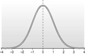 |
| Figure 35.1 Normal distribution showing standard deviations. |
If we wanted to go beyond simply calculating a set of sample statistics and wanted to know about the true mean value in the population – without having access to the whole population – we could take repeated (and different) samples from the first one we used and, for each of these, calculate a sample mean and standard deviation. Clearly, not all the means will be the same: they will be distributed about the population mean and it is this distribution from which we obtain the standard error of the mean. We do not have to carry out the tedious procedure of taking repeated samples; using our sample statistic, the standard deviation, we can calculate the standard error of the mean as shown:
 where N = number of subjects.
It should be noted that the standard deviation and the standard error are different statistics with different properties; the easiest level at which to differentiate them is that the standard deviation refers to a sample – unless you have the whole population available – and the standard error refers to the population – they are often confused (Altman & Bland 2005).
The standard error of the mean is used to calculate confidence intervals, which are usually quoted at 95% indicating that 95% of all the calculated sample means will fall within the range of the confidence interval. We know that the sample means are normally distributed; therefore, we can use this property to find the correct number from a table of values for the normal distribution corresponding to 95% confidence. The number is 1.96 (for the purposes of this chapter you do not need to know more about how this number is obtained) and this is used in the calculation of the confidence interval as shown:
Therefore, taking the example of blood glucose, if we sample a group of 20 people and calculate their mean blood glucose to be 5 mmol/l with a standard deviation of 1 mmol/l, we can calculate the standard error of the mean to be:
 and enter this into the equation for calculating the confidence interval at 95%, thus:
That is:
 which gives a 95% confidence interval of 4.55 to 5.45 mmol/l blood glucose, meaning that 95% of the samples we take will have a mean within that range.
If we want to be more confident, say 99% confident, we can calculate 99% confidence intervals and find the value in our tables of the normal distribution relating to 99% probability (this value is 2.58). Entering this into the equation for calculating confidence intervals gives us a 99% confidence interval from 2.42 to 7.58 mmol/l blood glucose. We see that the confidence interval is wider; i.e. the more confident we are about where the mean lies the less certain we know precisely what it is, i.e. the less accurate we are. This seeming paradox can be illustrated by asking someone to estimate the distance between their head and the ceiling. They may be able to give the distance to the nearest metre with a high degree of confidence but if you then ask them to estimate the distance to the ceiling to the nearest centimetre they will be less confident in their estimation – the more accurate they are required to be, the less confident they are in their estimate.
Confidence intervals can also be calculated for differences between means and for statistical tests such as odds ratios (Gardner & Altman 2000). This takes us beyond the scope of the present chapter but you are advised to consider the use of confidence intervals whenever possible as they are more informative than just the mean value (Watson et al 2006).
Statistical significance
In statistical terms, to say that something is significant has a particular meaning. For instance, if the outcome of a clinical trial is that one drug is statistically significantly better than another, this means there is a difference in their performance and that this is known at a particular level of statistical significance, usually p < 0.05. What we are doing is ascribing a level of probability to the outcome, which means the extent to which that outcome has happened by chance; in the case of p < 0.05 this means that there is a probability of less than one in 20 that the observed result has happened by chance (Hinton 1995). In other words, the result that we are observing is likely to have happened as a result of the phenomenon that we are measuring. In the example of the drug trial above we are stating how likely we think it is that the difference in the performance of one drug over another happened by chance and not as a result of some property of the drug. If the result were significant at p < 0.1 it would mean that there was a 1 in 10 probability that this would have happened by chance and if the result were significant at p < 0.01 it would be one in 100. The application of the concept of statistical significance will be exemplified in the inferential statistical tests described below.
The use of statistical significance enables us to avoid something called type I error and this means that we do not ascribe statistical significance to a result too readily (Watson et al 2006). We will meet another concept, type II error, towards the end of the chapter.
Statistical significance does not, necessarily, indicate that a result is clinically significant. It is possible to obtain statistical significance, for example, in a study of the action of two drugs, where the actual difference between the effectiveness of the drugs is very small and would, in fact, not confer any clinical advantage. Therefore, the actual size of the difference needs to be calculated. In the case of tests of association between two variables – to be described below – the same thing applies and how to do this will be described. Confidence intervals for the difference between two means is also useful in showing how big a difference really is (Gardner & Altman 2000). Clinical judgement is always required in conjunction with statistical tests.
Differences between means
One of the common uses of inferential statistics is in the study of differences between means as exemplified by the study of the effect of drugs in a clinical trial described above. There are three ways in which the difference between means can be tested and these involve:
▪ the difference between a mean value obtained from a study and the population mean for the same measurement;
▪ the mean difference between two independent groups;
▪ the difference in means before and after an intervention.
The statistical test commonly used in such studies is the t-test, so called because statistical significance is obtained by calculating a value which, arbitrarily, has been labelled ‘t’.
Stay updated, free articles. Join our Telegram channel

Full access? Get Clinical Tree


