17
Standard scores and normal distributions
Standard scores (z scores)
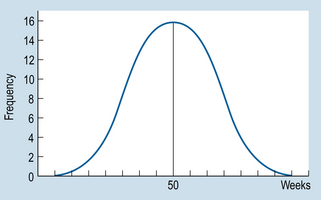
Consider this example: infant A walked unaided at the age of 40 weeks, while infant B is 65 weeks old but still cannot walk. What sense can we make of these measurements? Could infant B need further clinical investigation in case he has some neurological abnormality? The fact that infant B is unable to walk at the age of 65 weeks is not very informative in the absence of additional information about how this compares with norms for other children. However, say that it is known that the distribution of walking ages is such that µ = 50 weeks and σ = 5. Assuming that the frequency distribution is normal, the frequency polygon representing the population would look something like that shown in Figure 17.1.
A z score represents how many standard deviations a given raw score is above or below the mean. The equation for transforming specific raw scores into z scores is given as:
For the above equation, x is the raw score,  or µ is the mean of the distribution from which the score was drawn and s or σ is the standard deviation of the distribution. That is, when we know the mean and standard deviation of a distribution, we can transform any raw score into a z score. Conversely, when the z score is known, we can use the above equations to calculate the corresponding raw scores.
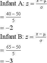
In the above example, the z scores corresponding to the infants’ raw scores are:
These calculations support our previous observations that A’s score was two standard deviations below the mean and B’s score was three standard deviations above the mean. In other words, A walked very early and B was a very late starter. The particular value of standardizing scores for understanding clinical or research evidence will be discussed in the context of the concepts of normal and standard normal distributions.
Normal distributions
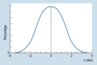
Many variables measured in the biological, behavioural and clinical sciences are approximately ‘normally’ distributed, i.e. they have a characteristic ‘bell-shaped’ curve. What is meant by a normal distribution is illustrated by the normal curve (see Fig. 17.2), which is a frequency polygon representing the theoretical distribution of population scores. We assume here that the variable x has been measured on an interval or ratio scale and that it is a continuous variable such as weight, height or blood pressure.
The normal curve has the following characteristics:
1. It is symmetrical about the mean, so that equal numbers of cases fall above and below the mean (mean = median = mode).
2. Relatively few cases fall into the high or low values of x. Most of the cases fall close to the mean. (For the theoretical normal distribution, the arms of the curve do not intersect with the x-axis, allowing for a few extreme scores.)
3. The precise equation for the normal curve was discovered by the mathematician Gauss, so that it is sometimes referred to as a Gaussian curve.
We need not worry about the actual formula for the normal curve. Rather, the point is that, given that the functional relationship between f and x is known, integral calculus can be used to calculate areas under the curve for any value of x. All normal curves have the same general mathematical form; whether we are graphing IQ or weight, the same bell shape will appear. The only differences between the curves are the mean value and the amount of variation. This is why the mean and the standard deviation provide us with important information about any particular normal distribution. Note that it is unlikely that any real data are exactly normally distributed. Rather, the normal distribution is a mathematical model that is useful for representing real distributions.
The standard normal curve
The standard normal curve has the following additional properties:
1. The mean is always 0 (zero). For the previous example, the z score corresponding to µ = 50 (as in the ‘infants’ walking age’ example) is:
2. The mean = median = mode, as the curve is symmetrical.
3. The standard deviation of z scores is always 1 (one). For instance, the z score for 55 (which is one standard deviation above the mean) is:
4. It is assumed that the total area under the curve adds up to 1.00. Since the normal curve is symmetrical, 0.5 of the area falls above z = 0 and 0.5 falls below z = 0. This is another way of saying that 50% of the total cases fall below the mean, and 50% of the cases fall above the mean (which is equal to the median).
5. More generally, we can use appropriate statistical tables to estimate the area under the standard normal curve for any given z scores. These areas are available in table form (see Appendix A) so that for any value of z we can read off the corresponding area.
6. The area under the curve between any two points is directly proportional to the percentage of cases falling above, below or between those two points. We can use the standard normal curve to calculate the percentage of scores falling between any specified two scores.
Stay updated, free articles. Join our Telegram channel

Full access? Get Clinical Tree


