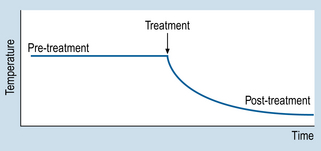
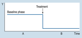
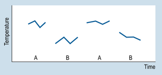
Let us assume that the drug is known to act quickly, say in 20 min. The evidence shown in Figure 9.1 would be clearly consistent with the hypothesis that the medication caused a decrease in the patient’s temperature. Let us generalize this example to n = 1 designs used in various settings. Figure 9.2 illustrates the general conventions used in n = 1 designs.

Figure 9.2 General structure of n = 1 designs.

1. We can see that the y-axis (Y) represents the outcome or dependent variable (DV): observations made of specific physical characteristics or behaviours.

2. The x-axis represents the time over which the observations were carried out.

3. The period A represents the sessions during which no intervention was administered. This is the ‘control’ level of the independent variable (IV). The observations recorded during A form the baseline.

4. Period B represents the sessions during which intervention was administered, i.e. the active stage.

5. The observations taken during A are compared with those taken during B. Systematic changes in the DV between A and B phases (increases or decreases) are assumed to reflect the influence of the intervention.

Therefore, an AB design involves taking observations during phase A, introducing an appropriate intervention, and then taking observations during B. It might have occurred to you that several of the threats to validity can be identified in AB designs. An obvious threat to validity is maturation: that is, recovery or deterioration occurring in the patient that might influence the readings on the outcome variable. Another possible threat is history: that is, influences on the patient other than the actual intervention. In the example we just looked at, one could also argue that perhaps the patient’s temperature would have gone down even without the drug, because of the condition improving by itself or the environment of the ward (maturation), or perhaps the ward was air-conditioned and the patient would have cooled down anyway, drugs or not (history).

Next, we look at ABAB designs, which provide stronger control for extraneous variables than AB designs.

ABAB designs

The basic feature of ABAB designs is the alternation of intervention with no-intervention or baseline phases. That is, the researcher introduces the intervention following a baseline or no-intervention phase, then the intervention is withdrawn and then re-introduced later. Observations are recorded during each phase and this approach permits control for the previously discussed threats to validity.

Figure 9.3 illustrates the outcomes for a hypothetical drug study using an ABAB design. When the drug is withdrawn (second A) the patient’s temperature returns to previous levels. When the drug is re-introduced (second B), the patient’s temperature declines. Clearly, such an outcome is consistent with a causal relationship between the independent variable (intervention) and the outcome or dependent variable (observations of temperature). Figure 9.4 demonstrates the idealized results expected using ABAB designs with a highly effective rapid-onset intervention.