19
Probability and confidence intervals
Introduction
Sample statistics (such as  , s) are estimates of the actual population parameters, in this case µ, σ. Even where adequate sampling procedures are adopted, there is no guarantee that the sample statistics are exactly the same as the true parameters of the population from which the samples were drawn. Therefore, inferences from sample statistics to population parameters necessarily involve the possibility of sampling error. As stated in Chapter 5, sampling errors represent the discrepancy between sample statistics (i.e. the results we obtain in a study sample) and true population parameters (i.e. what we would obtain if we accurately studied the whole population). Given that investigators usually have no knowledge of the true population parameters (because they are unable to study the entire population), inferential statistics are employed to estimate the probable sampling errors when using statistical data based on a study sample. While sampling error cannot be completely eliminated, the probable size of sampling error can be calculated using inferential statistics. In this way investigators are in a position to calculate the probability of being accurate in their estimations of the actual population parameters.
The aims of this chapter are to examine how probability theory is applied to generating sampling distributions and how sampling distributions are used for estimating population parameters. Sampling distributions are used to estimate sampling error. This statistic is then used to calculate confidence intervals as well as testing hypotheses (see Ch. 20).
The specific aims of this chapter are to:
Probability
The concept of probability is central to the understanding of inferential statistics. Probability is expressed as a proportion between 0 and 1, where 0 means an event is certain not to occur, and 1 means an event is certain to occur. Therefore if the probability (p) is 0.01 for an event then it is unlikely to occur (chance is 1 in 100). If p = 0.99 then the event is highly likely to occur (chance is 99 in 100). The probability of any event (say event A) occurring is given by the formula:
Sometimes the probability of an event can be calculated a priori (before the event) by reasoning alone. For example, we can predict that the probability of throwing a head (H) with a fair coin is:
Or, if we buy a lottery ticket in a draw where there are 100 000 tickets, the probability of winning first prize is:
In some situations, there are no theoretical grounds for calculating the occurrence of an event (a priori). For instance, how can we calculate the probability of an individual dying of a specific condition? In such instances, we use previously obtained evidence to calculate probabilities a posteriori (after the event).
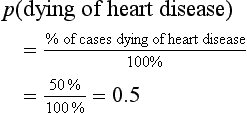
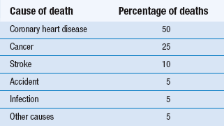
For example, if we have information for the mortality rates of a community (Table 19.1) we are in a position to calculate the probability of a selected individual over 65 years of age dying of any of the specified causes. For example, the probability of a given individual dying of coronary heart disease is:
Also, we can use the normal curve model, as outlined in Chapter 17, to determine the proportion or percentage of cases up to, or between, any specified scores. In this instance, probability is defined as the proportion of the total area cut off by the specified scores under the normal curve. As we discussed in Chapter 17, the greater the area under the curve, the higher the corresponding probability of selecting specified values.
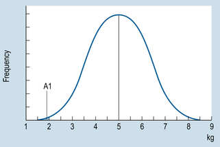
For example, say that Figure 19.1 illustrates the birth weights of a large sample of neonates. Let us assume that the distribution is approximately normal, with the mean ( ) of 5.0 kg and a standard deviation (s) of 1.5. We can use the information to calculate the probability of any range of birth weights. Now, say that we are interested in the probability of a randomly selected neonate having a birth weight of 2.0 kg or under.
The area A1 under the curve in Figure 19.1 corresponds to the probability of obtaining a score of 2 or under. Using the principles outlined in Chapter 17 to calculate proportions or areas under the normal curve, we first translate the raw score of 2 into a z score:
Now we look up the area under the normal curve corresponding to z = −2 (Appendix A). Here we find that A1 is 0.0228. This area corresponds to a probability, and we can say that ‘The probability of a neonate having a birth weight of 2 kg or less is 0.0228’. Another way of stating this outcome is that the chances are approximately 2 in 100, or 2%, for a child having such a birth weight.
We can also use the normal curve model to calculate the probability of selecting scores between any given values of a normally distributed continuous variable. For example, if we are interested in the probability of birth weights being between 6 and 8 kg, then this can be represented on the normal curve (area A2 on Fig. 19.2). To determine this area, we proceed as outlined in Chapter 15. Let s = 1.5.
Therefore the area between z1 and  is 0.2486 (from Appendix A) and the area between z2 and
  is 0.4772 (from Appendix A). Therefore, the required area A2 is:
It can be concluded that the probability of a randomly selected child having a birth weight between 6 and 8 kg is p = 0.2286. Another way of saying this is that there is a 23 in 100, or a 23%, chance that the birth weight will be between 6 and 8 kg.
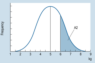
Figure 19.2 Frequency distribution of neonate birth weights. Area A2 corresponds to probability of weight being 6–8 kg.
Sampling distributions
Given the above population, say that samples of marbles are drawn randomly and with replacement. (By ‘replacement’ we mean the samples are put back into the population, in order to maintain as a constant the proportion of B = W = 0.5.) If we draw samples of four (i.e. n = 4) then the possible proportions of black and white marbles in the samples can be deduced a priori as shown in Figure 19.3.
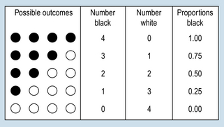
Figure 19.3 Characteristics of possible samples of n = 4, drawn from a population of black and white marbles.
Ignoring the order in which marbles are chosen, Figure 19.3 demonstrates all the possible outcomes for samples of sample size n = 4. It is logically possible to draw any of the samples shown. However, only one of the samples (2B, 2W), is representative of the true population parameter. The other samples would generate incorrect inferences concerning the state of the population. In general, if we know or assume (hypothesize) the true population parameters, we can generate distributions of the probability of obtaining samples of a given characteristic.
P is the probability of the first outcome, Q is the probability of the second outcome and n is the number of trials (or the sample size).
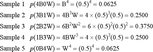
The following shows the composition of the samples which can be drawn from the specified population and the probability of obtaining a specific sample. For the present case:
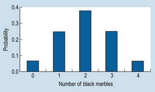
The calculated probabilities add up to 1, indicating that all the possible sample outcomes have been accounted for (because the probability of all possible events must equal 1.0). However, the important issue here is not so much the mathematical details but the general principle being illustrated by the example. For a given sample size (n) we can employ a mathematical formula to calculate the probability of obtaining all the possible samples from a population with known characteristics. The relationship between the possible samples and their probabilities can be graphed, as shown in Figure 19.4.
Stay updated, free articles. Join our Telegram channel

Full access? Get Clinical Tree


