8.1 Back to basics
Before going any further I want to stop and explain some statistical terminology. Understanding the plethora of terms is half the battle in overcoming a fear of statistics. As the title states, this section takes you right back to basic maths; some readers will find this a helpful starter, for many this will be valuable revision but some may like to skip through to Section 8.2. Before you decide to skip on why don’t you test yourself using the ‘test questions’ at the start of each section? These questions summarise what each section will tell you and enable you to find out what you really know!
8.1.1 Populations and samples
Test question: Give some examples of populations and samples.
The purpose of statistical analysis in health and social research is to use information about a sample of individuals to make inferences about the wider population. A sample is a selected group from the population of interest. Generally we are talking about people but it can be a sample of anything. For example, a study about A & E service provision may use a sample of 50 hospitals from the total ‘population’ of NHS Hospitals in the UK. This, you may be thinking, is obvious but it is always important to remember the underlying principles when interpreting and carrying out analyses.
8.1.2 Probability
Test question: Explain probability and why is it an important concept in statistics?
The probability of an event happening is the proportion of times the event would occur if we repeated the experiment a large number of times. This is usually expressed as a percentage or a decimal, for example, the probability of throwing 1 when tossing a dice is 1/6, 17% or 0.17. A probability of 0 means there is no chance of that event happening (probability of throwing 7), and a probability of 1 means a particular event will always happen (probability of throwing 1, 2, 3, 4, 5, or 6). You need to understand probability since this is the basis of inferential statistics.
8.1.2.1 p values
When you come to analyse data you are no doubt expecting to produce some p values; p stands for probability, and is telling you the probability of the hypothesis you are testing occurring by chance alone. As Altman (1999) states in his statistical textbook, ‘Statistical analysis allows us to put limits on our uncertainty, but not to prove anything’. Statistics is all about probability.
8.1.3 Types of data
Test questions: What is the difference between continuous and discrete data? What is the difference between ordinal and nominal data? Give examples of each type.
There are various different types of data and each is analysed using different methods. Identifying which type of data you will produce in your study is the first step in planning how you will analyse it.
8.1.3.1 Numerical data
Continuous data are generally acquired using some sort of measurement and are not limited to a fixed set of values. Examples include age, weight, height, distance travelled for health care or blood sugar level. In each case, any value is possible between the biological norms, so for humans you could get values of age between 0 and say 115 years, and the precision of the measurement depends on the requirements of the particular study (whether it is in days, months or years).
Discrete data can take a value from a finite set of possible values. They are often analysed as continuous but sometimes may be better analysed using other methods. Examples include number of appointments, number of children, age at last birthday or shoe size. It is not possible to have half an appointment or 0.3 of a child and this is what distinguishes this type of data from continuous.
8.1.3.2 Categorical data
Categorical data is where the observation made can only be one option, in other words values are categorised into two or more groups. There are two main types of categorical data: ordinal and nominal. Ordinal data have a meaningful order, such as a 5 point pain scale or social class. It is important to note that you cannot assume the interval between each ordered category is the same (i.e. someone scoring 4 on a pain scale does not necessarily have twice as much pain as someone scoring 2) and this makes ordinal data different to discrete numerical data. Nominal data have no order and examples include ethnicity or blood group. Nominal data also include a special case: binary or dichotomous data, which have only two possible categories such as gender, disease or no disease and in-patient or out-patient.
8.1.4 Describing your data
There are several terms you will come across regularly when reading quantitative research papers and you will need to be able to use this terminology when you come to describing your own data. You are likely to have heard of many of the following terms but perhaps you can’t actually define them. As before test yourself as you go through this section and see how much you do know or where you need more revision.
8.1.4.1 Central tendency or average
Test question: What are the three ways to describe the average value of a set of data and how do you calculate them?
There are three ways to describe the average of a set of data and which you use depends on the type of data you have. The three ways are mean, median and mode. The mean is the sum of all the observations in the data set divided by the number of observations, and this is the value usually referred to when people talk about the ‘average’. The median is the middle observation when they are listed in order of increasing size. If you have an even number of observations you will have two ‘middle’ values and in this case you would take the mean of these two values to calculate the median. Finally the mode is the most frequently observed value in any given set of data. This is the least used of the three types of ‘averages’ but can be useful for discrete data.
8.1.4.2 Variation in the data
Test question: What measures of variation are there and how would you describe them?
There are three main ways to describe the variation seen in any given set of data and again which you use will depend on the data. The three ways are the range, the inter-quartile range and the standard deviation. The range is simply the maximum and minimum values. This represents the total spread of the data but tells you little about how each individual value varies from the others. This makes the range less useful but it is sometimes of value to quote it if you wish to describe the total spread of the data.
The inter-quartile range (IQR) includes the values between which the middle 50% of the data lie, or put another way are the values at the 25% and 75% percentiles. This means the values below which 25% and 75% of the data lie. The median is at the 50th centile since half the data lie below and half above this value. The inter-quartile range is useful since it describes the middle bulk of the data and excludes the increasingly extreme outlying values. A larger difference between these two values illustrates the greater variation in the data and this measure of variation is commonly used with the median.
The standard deviation (SD, sd, s, or o) is calculated using a specific formula and provides a single figure to show the amount of variation within a set of data. A larger standard deviation equates to more variation within the set of data.
8.1.4.3 Data distributions
Test question: What kind of distributions are there and what type of average and measure of variation is most appropriate to use with these distributions?
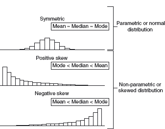
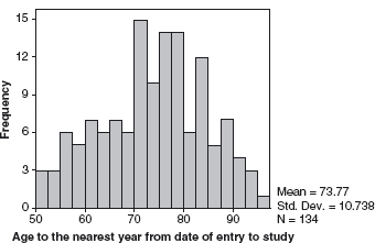
You may well now be wondering how you decide which of these ‘averages’ or ‘measures of variation’ you should choose to use. It all pivots on the distribution of your data. Figure 8.1 shows histograms illustrating three main types of data distribution in a pure form. Obviously clinical data will never be this pure and your distribution will approximate to one or other of these types. There are several ways to find out how your data are distributed but one of the easiest is to plot a histogram and look at it. Does it look roughly normal or is it more skewed one way or the other? Figure 8.2 gives an example of a histogram plotted for a group of 134 patients aged over 50 years. If you look at the horizontal axis you will see each column covers a range of 2.5 years, thus this diagram tells you that three patients were aged between 50 and 52.5 years and that one was aged between 95 and 97.5 years. This histogram shows an approximately normal distribution. Histograms are very easily generated on computer statistical software so don’t worry about creating such diagrams.
Figure 8.1 Three main types of data distribution.

Figure 8.2 Histogram showing the age distribution in a study looking at adults over 50 years.

These distribution types are described as either normal (parametric) or skewed (non-parametric). If you read more about statistics you find several other distributions described but I am sticking to the basics here and for more detail you will need to turn to a specialist source. Looking again at Figure 8.1 will show you that the values of the different types of averages vary depending on the distribution of the data. For normal data all averages will be similar but for skewed data there are considerable differences between the mean, median and mode. For normal data the best measure to use is the mean since every value contributes to the calculation of the mean. For skewed data the best description of the central tendency is the median. The best descriptors of the amount of variation are the inter-quartile range for skewed data and standard deviation for normal data.
8.1.5 Using your data to answer your research question
We have now covered the basics for describing your data and I will move on to look at analysis. The purpose of descriptive statistics is to describe the characteristics of the study sample and you can then see how the sample fits with the general population of interest. However, to test hypotheses you need to use what are termed inferential statistics; put simply you are using a small sample to make inferences or draw conclusions about a larger population. Do not panic about carrying out such calculations; at this stage it is far more important to understand the principles involved and the terminology used. Actually carrying out the analysis will come later.
8.1.5.1 Hypothesis testing
Test questions: What is a null hypothesis? What does a p value of 0.05 mean?
As described earlier (see Chapter 7, Section 7.2.4), when you set up a study you have a research question which can also be phrased as a statement or hypothesis. This can then be re-phrased as a NULL hypothesis (H0), and an example is given in Section 7.2.4. In using statistics we are trying to show the likelihood that the null hypothesis is true. Once you have defined your null hypothesis you test it using the appropriate statistical test and calculate a p value (remember p = probability). This tells you the probability of your study yielding its findings if the null hypothesis is true; or how likely were you to get these results through chance alone. For example, put simply, if you obtain a p value of 0.05 this means there is 5% chance that the null hypothesis is true or 95% chance it is wrong.
Table 8.1 A comparison of the total number of cases of antibiotic associated diarrhoea in each study group.

Stay updated, free articles. Join our Telegram channel

Full access? Get Clinical Tree


