18
Correlation
Introduction
A fundamental aim of scientific and clinical research is to establish the nature of the relationships between two or more sets of observations or variables. Finding such relationships or associations can be an important step for identifying causal relationships and the prediction of clinical outcomes. The topic of correlation is concerned with expressing quantitatively the size and the direction of the relationship between variables. Correlations are essential statistics in the health sciences, used to quantitatively determine the validity and reliability of clinical measures (see Ch. 14) or expressing how health problems are associated with crucial biological, behavioural or environmental factors (see Ch. 8). Having worked through this chapter you will be able to explain how correlation coefficients are used and interpreted in health sciences research and practice.
The specific aims of this chapter are to:
1. Define the terms correlation and correlation coefficient.
2. Explain the selection and calculation of correlation coefficients.
3. Outline some of the uses of correlation coefficients.
4. Define and calculate the coefficient of determination.
5. Discuss the relationship between correlation and causality.
Correlation
Consider the following two statements:
1. There is a positive relationship between cigarette smoking and lung damage.
2. There is a negative relationship between being overweight and life expectancy.
You probably have a fair idea what the above two statements mean. The first statement implies that there is evidence that if you score high on one variable (cigarette smoking) you are likely to score high on the other variable (lung damage). The second statement describes the finding that scoring high on the variable ‘overweight’ tends to be associated with lowered ‘life expectancy’. The information missing from each of the statements is the numerical value for size of the association between the variables.
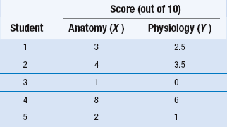
Assume that we are interested to see whether student test scores for anatomy examinations are correlated with test scores for physiology. To keep the example simple, we will assume that there were only five (n = 5) students who sat for both examinations (see Table 18.1).
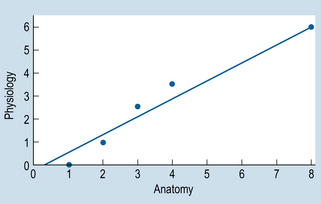
To provide a visual representation of the relationship between the two variables, we can plot the above data on a scattergram (also referred to as a scatterplot). A scattergram is a graph of the paired scores for each participant on the two variables. By convention, we call one of the variables x and the other one y. It is evident from Figure 18.1 that there is a positive relationship between the two variables. That is, students who have high scores for anatomy (variable X) tend to have high scores for physiology (variable Y). Also, for this set of data, we can fit a straight line in close approximation to the points on the scattergram. This line is referred to as a line of ‘best fit’. This topic is discussed further in statistics under ‘linear regression’. In general, a variety of relationships is possible between two variables; the scattergrams in Figure 18.2 illustrate some of these.

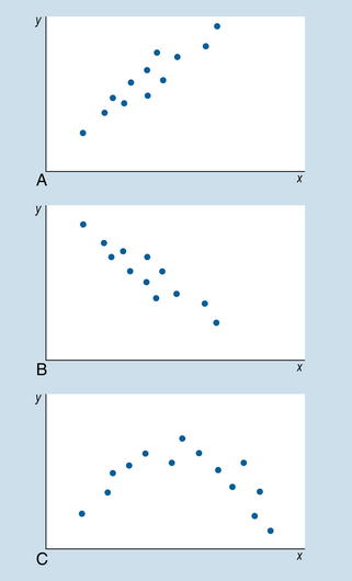
Figure 18.2 Scattergrams showing relationships between two variables: (A) positive linear correlation; (B) negative linear correlation; (C) non-linear correlation.
Figure 18.2A and B represent a linear correlation between the variables x and y. That is, a straight line is the most appropriate representation of the relationship between x and y. Figure 18.2C represents a non-linear correlation, where a curve best represents the relationship between x and y.
Figure 18.2A represents a positive correlation, indicating that high scores on x are related to high scores on y. For example, the relationship between cigarette smoking and lung damage is a positive correlation. Figure 18.2B represents a negative correlation, where high scores on x are associated with low scores on y. For example, the correlation between the variables ‘being overweight’ and ‘life expectancy’ is negative, meaning that the more you are overweight, the lower your life expectancy.
Correlation coefficients
Selection of correlation coefficients
There are several types of correlation coefficients used in statistical analysis. Table 18.2 shows some of these correlation coefficients, and the conditions under which they are used. As the table indicates, the scale of measurements used determines the selection of the appropriate correlation coefficient.
Table 18.2
| Coefficient | Conditions where appropriate |
| φ (phi) | Both x and y measures on a nominal scale |
| ρ (rho) | Both x and y measures on, or transformed to, ordinal scales |
| r | Both x and y measures on an interval or ratio scale |
All of the correlation coefficients shown in Table 18.2 are appropriate for quantifying linear relationships between variables. There are other correlation coefficients, such as η (eta) which are used for quantifying non-linear relationships. However, the discussion of the use and calculation of all the correlation coefficients is beyond the scope of this text. Rather, we will examine only the commonly used Pearson’s r, and Spearman’s ρ (rho).
1. Correlation coefficients are calculated from pairs of measurements on variables x and y for the same group of individuals.
2. A positive correlation is denoted by + and a negative correlation by −.
3. The values of the correlation coefficient range from +1 to −1, where +1 means a perfect positive correlation, 0 means no correlation, and −1 a perfect negative correlation.
4. The square of the correlation coefficient represents the coefficient of determination.
Stay updated, free articles. Join our Telegram channel

Full access? Get Clinical Tree


